CMSC 425 Lecture Notes - Lecture 15: Perlin Noise, Tangent Space, Stochastic Process

15 May 2018
School
Department
Course
Professor

CMSC 425 Dave Mount & Roger Eastman
CMSC 425: Lecture 13
Procedural Generation: 2D Perlin Noise
Reading: The material on Perlin Noise based in part by the notes Perlin Noise, by Hugo Elias.
(The link to his materials seems to have been lost.)
Perlin Noise in 2D: In the previous lecture we introduced the concept of Perlin noise, a struc-
tured random function, in a one-dimensional setting. In this lecture we show how to generalize
this concept to a two-dimensional setting. Such two-dimensional noise functions can be used
for generating pseudo-random terrains and two-dimensional pseudo-random textures.
The general approach is the same as in the one-dimensional case:
•Generate a finite sample of random values
•Generate a noise function that interpolates smoothly between these values
•Sum together various octaves of this function by scaling it down by factors of 1/2, and
then applying a dampening persistence value to each successive octave, so that high
frequency variations are diminished
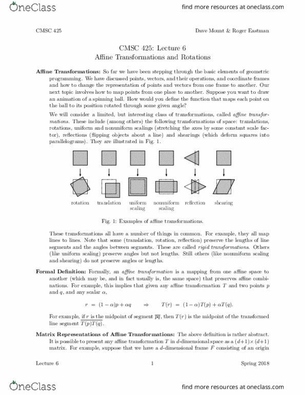
Let’s investigate the finer points. First, let us begin by assuming that we have an n×ngrid of
unit squares (see Fig. 1(a)), for a relatively small number n(e.g., nmight range from 2 to 10).
For each vertex [i, j] of this grid, where 0 ≤i, j ≤n, let us generate a random scalar value
z[i,j]. (Note that these values are actually not very important. In Perlin’s implementation of
the noise function, these value are all set to 0, and it still produces a remarkably rich looking
noise function.) As in the 1-dimensional case, it is convenient to have the values wrap around,
which we can achieve by setting z[i,n]=z[i,0] and z[n,j]=z[0,j]for all iand j.
Given any point (x, y), where 0 ≤x, y < n, the corner points of the square containing this
point are (x0, y0), (x1, y0), (x1, y1), (x0, y1) where:
x0=bxcand x1= (x0+ 1) mod n
y0=bycand y1= (y0+ 1) mod n
(see Fig. 1(a)).
We could simply apply smoothing to the random values at the grid points, but this would
produce a result that clearly had a rectangular blocky look (since every square would suffer the
same variation). Instead, Perlin came up with a way to have every vertex behave differently,
by creating a random gradient at each vertex of the grid.
Noise from Random Gradients: Before explaining the concept of gradients, let’s recall some
basics from differential calculus. Given a continuous function f(x) of a single variable x, we
know that the derivative of the function df/dx yields the tangent slope at the point (x, f(x))
on the function. If we instead consider a function f(x, y) of two variables, we can visualize the
function values (x, y, f(x, y)) as defining the height of a point on a two-dimensional terrain. If
fis smooth, then each point of the terrain can be associated with tangent plane. The “slope”
of the tangent plane passing through such a point is defined by the partial derivatives of the
Lecture 13 1 Spring 2018

CMSC 425 Dave Mount & Roger Eastman
(x, y)
0
1
n
0
1
n
(x0, y1)
(x0, y0)
(x1, y0)
(x1, y1)
(a)
0
1
n
0
1
n
(b)
Initial grid
Random gradient vectors
g[0,1]
g[0,0]
g[1,1]
g[1,0]
v[0,1]
v[0,0]
v[1,0]
v[1,1]
(c)
Smoothing/Interpolation
Fig. 1: Generating 2-dimensional Perlin noise.
function, namely ∂f/∂x and ∂f/∂y. The vector (∂f/∂x, ∂f/∂y) is a vector in the (x, y)-plane
that points in the direction of steepest ascent for the function f. This vector changes from
point to point, depending on f. It is called the gradient of f, and is often denoted ∇f.
Perlin’s approach to producing a noisy 2-dimensional terrain involves computing a random 2-
dimensional gradient vector at each vertex of the grid with the eventual aim that the smoothed
noise function have this gradient value. Since these vectors are random, the resulting noisy
terrain will appear to behave very differently from one vertex of the grid to the next. At one
vertex the terrain may be sloping up to the northeast, and at a neighboring vertex it may be
slopping to south-southwest. The random variations in slope result in a very complex terrain.
But how do we define a smooth function that has this behavior? In the one dimensional
case we used cosine interpolation. Let’s consider how to generalize this to a two-dimensional
setting.
Consider a single square of the grid, with corners (x0, y0), (x1, y0), (x1, y1), (x0, y1). Let g[0,0],
g[1,0],g[1,1], and g[0,1] denote the corresponding randomly generated 2-dimensional gradient
vectors (see Fig. 1(c)). Now, for each point (x, y) in the interior of this grid square, we need to
blend the effects of the gradients at the corners. To do this, for each corner we will compute
a vector from the corner to the point (x, y). In particular, define
v[0,0] = (x, y)−(x0, y0) and v[0,1] = (x, y)−(x0, y1)
v[1,0] = (x, y)−(x1, y0) and v[1,1] = (x, y)−(x1, y1)
(see Fig. 1(c)).
Next, for each corner point of the square, we generate an associated vertical displacement,
which indicates the height of the point (x, y) due to the effect of the gradient at this corner
point. How should this displacement be defined? Let’s fix a corner, say (x, 0, y0). Intuitively,
if v[0,0] is directed in the same direction as the gradient vector, then the vertical displacement
will increase (since we are going uphill). If it is in the opposite direction, the displacement
will decrease (since we are going downhill). If the two vectors are orthogonal, then the vector
v[0,0] is directed neither up- or downhill, and so the displacement is zero. Among the vector
Lecture 13 2 Spring 2018
Document Summary
Reading: the material on perlin noise based in part by the notes perlin noise, by hugo elias. (the link to his materials seems to have been lost. ) Perlin noise in 2d: in the previous lecture we introduced the concept of perlin noise, a struc- tured random function, in a one-dimensional setting. In this lecture we show how to generalize this concept to a two-dimensional setting. Such two-dimensional noise functions can be used for generating pseudo-random terrains and two-dimensional pseudo-random textures. First, let us begin by assuming that we have an n n grid of unit squares (see fig. 1(a)), for a relatively small number n (e. g. , n might range from 2 to 10). For each vertex [i, j] of this grid, where 0 i, j n, let us generate a random scalar value z[i,j]. (note that these values are actually not very important.