CMSC 425 Lecture Notes - Lecture 73: Fractal Dimension, Mandelbrot Set, Julia Set

15 May 2018
School
Department
Course
Professor

CMSC 425 Dave Mount & Roger Eastman
CMSC 425: Lecture 11
Procedural Generation: Fractals and L-Systems
Reading: The material on fractals comes from classic computer-graphics books. The material on
L-Systems comes from Chapter 1 of The Algorithmic Beauty of Plants, by P. Prunsinkiewicz and
A. Lindenmayer, 2004. It can be accessed online from http://algorithmicbotany.org/papers/.
Fractals: One of the most important aspects of any graphics system is how objects are modeled.
Most man-made (manufactured) objects are fairly simple to describe, largely because the
plans for these objects are be designed “manufacturable”. However, objects in nature (e.g.
mountainous terrains, plants, and clouds) are often much more complex. These objects are
characterized by a nonsmooth, chaotic behavior. The mathematical area of fractals was
created largely to better understand these complex structures.
One of the early investigations into fractals was a paper written on the length of the coastline
of Scotland. The contention was that the coastline was so jagged that its length seemed to
constantly increase as the length of your measuring device (mile-stick, yard-stick, etc.) got
smaller. Eventually, this phenomenon was identified mathematically by the concept of the
fractal dimension. The other phenomenon that characterizes fractals is self similarity, which
means that features of the object seem to reappear in numerous places but with smaller and
smaller size.
In nature, self similarity does not occur exactly, but there is often a type of statistical self
similarity, where features at different levels exhibit similar statistical characteristics, but at
different scales.
Iterated Functions and Attractor Sets: One of the examples of fractals arising in mathemat-
ics involves sets called attractors. The idea is to consider some function of space and to see
where points are mapped under this function. An elegant way to do this in the plane is to
consider functions over complex numbers. Each coordinate (a, b) in the real plane is asso-
ciated with the complex number a+bi, where i2=−1. Adding and multiplying complex
numbers follows the familiar rules:
(a+bi)+(c+di)=(a+c)+(b+d)i,
and
(a+bi)(c+di) = ac +adi +bci +bdi2= (ac −bd)+(ad +bc)i.
Define the modulus of a complex number a+bi to be length of the corresponding vector in
the complex plane, √a2+b2. This is a generalization of the notion of absolute value with
reals. Observe that the numbers of given fixed modulus just form a circle centered around
the origin in the complex plane.
Now, consider any complex number z0= (a0+b0i)∈C. If we repeatedly square this number,
zi←z2
i−1, for i= 1,2,3, . . .. then it is easy to verify that with each step the modulus is
also squared. If the modulus of z0is strictly smaller than 1, then the resulting sequence of
complex numbers will become smaller and smaller (in terms of their moduli) and hence will
converge to the origin in the limit. If the modulus of z0is strictly larger than 1, the moduli
Lecture 11 1 Spring 2018

CMSC 425 Dave Mount & Roger Eastman
will grow to infinity, implying that the sequence will move arbitrarily far from the origin.
Finally, if the modulus is equal to 1, it will remain so, and the sequence will spiral around
the unit circle.
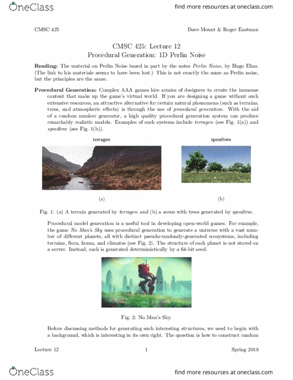
In general, we can do this using any function f:C→Con the complex plane. We define the
attractor set (or fixed-point set ) to be a subset of nonzero points that remain fixed under the
mapping. Note that it is the set as a whole that is fixed, even though the individual points
tend to move around (see Fig. 1).
Fig. 1: An iterated function. The subset within the blue region converges to the origin. The
attractor set (the black curved boundary) is preserved under the function.
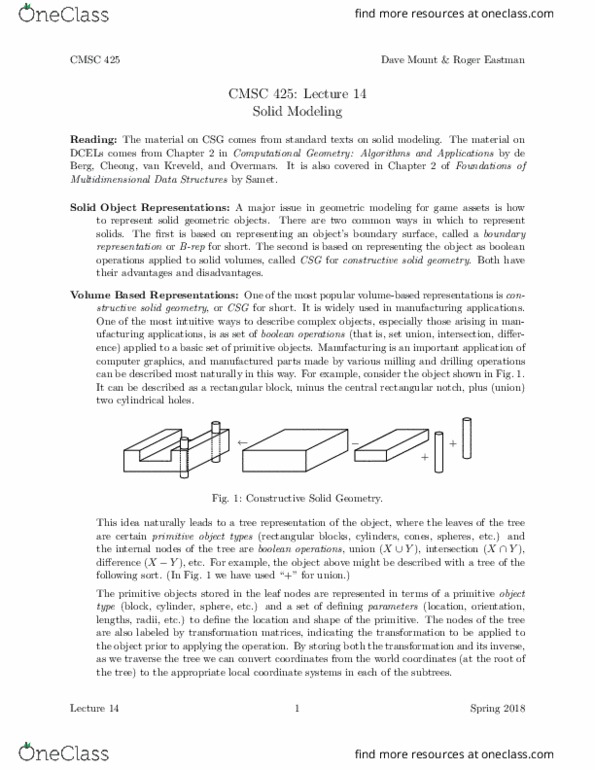
Julia and Mandelbrot Sets: For any complex constant c∈C, consider the iterated function
zi←z2
i−1+cfor i= 1,2,3, . . .
Now as before, under this function, some points will tend toward ∞and others towards finite
numbers. However there will be a set of points that will tend toward neither. Altogether
these latter points form the attractor of the function system. This is called the Julia set for
the point c. An example of such a set is shown in Fig. 2(a).
(a)
(b)
Fig. 2: (a) a Julia set and (b) the Mandelbrot set.
Lecture 11 2 Spring 2018

CMSC 425 Dave Mount & Roger Eastman
A common method for approximately rendering Julia sets is to iterate the function until the
modulus of the number exceeds some prespecified threshold. If the number diverges, then we
display one color, and otherwise we display another color. How many iterations? It really
depends on the desired precision. Points that are far from the boundary of the attractor will
diverge quickly. Points that very close, but just outside the boundary may take much longer
to diverge. Consequently, the longer you iterate, the more accurate your image will be.
For some complex numbers cthe associated Julia set forms a connected set of points in the
complex plane. For others it is not. For each point cin the complex plane, if we color it black
if Julia(c) is connected, and color it white otherwise, we will a picture like the one shown
below. This set is called the Mandelbrot set (see Fig. 2(b)).
Fractal Dimension: One of the important elements that characterizes fractals is the notion of
fractal dimension. Fractal sets behave strangely in the sense that they do not seem to be 1-,
2-, or 3-dimensional sets, but seem to have noninteger dimensionality.
What do we mean by the dimension of a set of points in space? Intuitively, we know that
a point is zero-dimensional, a line (or generally a curve) is one-dimensional, and plane (or
generally a surface) is two-dimensional, and so on. If you put the object into a higher
dimensional space (e.g., a line in 5-space) it does not change the dimensionality of the object,
it is still a 1-dimensional set. If you continuously deform an object (e.g. deform a line into a
circle or a plane into a sphere) it does not change its dimensionality.
How do you define the dimension of a set in general? There are various methods. Here is
one, which is called fractal dimension. Suppose we have a set in d-dimensional space. Define
ad-dimensional ε-ball to the interior of a d-dimensional sphere of radius ε. An ε-ball is an
open set (it does not contain its boundary) but for the purposes of defining fractal dimension
this will not matter much. In fact it will simplify matters (without changing the definitions
below) if we think of an ε-ball to be a solid d-dimensional hypercube whose side length is 2ε
(an ε-square).
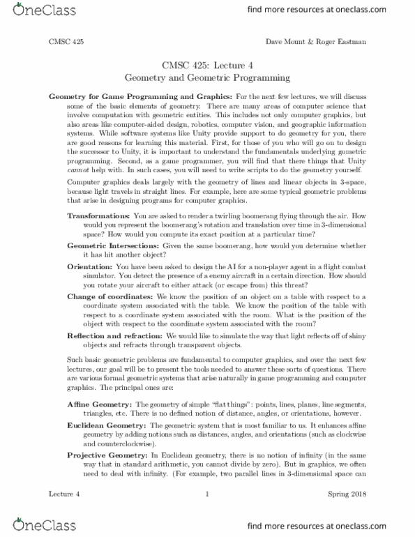
The dimension of an object depends intuitively on how the number of balls its takes to cover
the object varies with ε. First consider the case of a line segment. Suppose that we have
covered the line segment with n ε-balls. If we decrease the size of the covering balls exactly
by 1/2, it is easy to see that it takes roughly twice as many, that is, 2n, to cover the same
segment (see Fig. 3(a)).
n
2n
(a)
n
4n
(b)
Fig. 3: The growth rate of covering numbers and fractal dimension.
Next, let’s consider a square that has been covered with n ε-balls. If we decrease the radius
by 1/2, we see that its now takes roughly four times, that is, 4n, as many balls (see Fig. 3(b)).
Lecture 11 3 Spring 2018
Document Summary
Reading: the material on fractals comes from classic computer-graphics books. L-systems comes from chapter 1 of the algorithmic beauty of plants, by p. prunsinkiewicz and: lindenmayer, 2004. Fractals: one of the most important aspects of any graphics system is how objects are modeled. Most man-made (manufactured) objects are fairly simple to describe, largely because the plans for these objects are be designed manufacturable . However, objects in nature (e. g. mountainous terrains, plants, and clouds) are often much more complex. These objects are characterized by a nonsmooth, chaotic behavior. The mathematical area of fractals was created largely to better understand these complex structures. One of the early investigations into fractals was a paper written on the length of the coastline of scotland. The contention was that the coastline was so jagged that its length seemed to constantly increase as the length of your measuring device (mile-stick, yard-stick, etc. ) got smaller.