STAT 2000 Lecture Notes - Lecture 3: Pie Chart

23 Feb 2017
School
Department
Course
Professor

January 18, 2017
Chapter 2 Continued
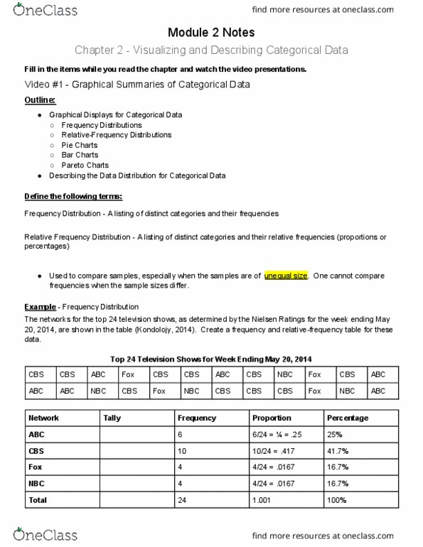
• Frequency tables: easy way to summarize data (usually categorical)
• Bar graphs: categories on horizontal axis
• Pareto Chart: ordered by frequencies from tallest bar to shortest
o Categories in descending order; vertical axis shows proportion in each category
• Pie chart: circle divided into sections; each section = category
• Contingency Table: used to show how two categorical variables relate
• Conditional Distributions: restrict variables to show distribution for just those cases that
satisfy a specified condition
• Independence
o Distribution of one variable is the same for all categories of another
variable=independent
o Heights of graphs=same height (i.e. gender and handedness)
2.2 Graphs for Quantitative Variables
• Dot Plot: a dot for each piece of data
o # of dots=sample size
• Histograms: uses bars to portray frequency of possible outcomes
o Horizontal axis (x) represents the values the variable can take on
o Vertical axis (y) represents how many of each value falls within a certain range of
variables
o Height of rectangles in graph=frequency of groups on chart
• EX. 8 IQ Squares
o 1. How many students sampled? 205; add frequencies
o 2. Bar with the highest frequency? Number of observations
▪ 100-109; 98
o 3. Bar with the fewest frequency? Number of observations
▪ 140-149; 1
o 4. Proportion of students with an IQ 120-129
▪ 12/205
o 5. Shape of distribution
▪ bell curve
▪ normal distribution
▪ one peak
▪ mount shape
▪ symmetric
• The shape of a histogram describes the distribution
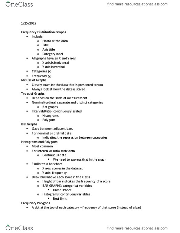
2.3 Measuring the Center of Quantitative Data
• Most frequent used measures of center= mean and median
o Mean (average): sum of observation divided by the # of observers
o Median (middle): observations ordered from smallest to largest, median splits it in
two; half below and half above
find more resources at oneclass.com
find more resources at oneclass.com