GEOG 371 Lecture Notes - Lecture 14: Spurious Relationship, Ecological Fallacy, Dependent And Independent Variables

5 May 2018
School
Department
Course
Professor

Week 14
4/16
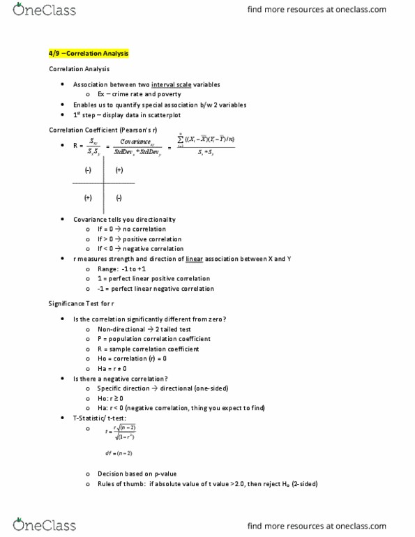
Correlation Analysis
• Chi square – 2 nominal variables
• “peara’s r – 2 ordinal variables
o Ranked
o Small n (n < 20)
• Pearso’s r – 2 interval variables
Issues in Correlation Analysis
• Always check scatterplot
o Always map your data too
• Spurious correlation
o Correlation that exists but does not make any logical sense
• Correlation does not imply causation
• Geographical scale of data affects correlation
o Correlation tends to increase where area/ population size increases
• Ecological fallacy
Linear Regression Analysis
• Response variable (Dependent variable) – Y
• Predictor variable (Independent variable) – X
• Respose ariale respods to the preditor ariale. X results i a hage i Y
• Ex – crime (y), poverty (x)
o If people live in poverty they may respond to that by committing crime (or are victims of
crime)
• Equation:
•
o e = error term
o a = y int
o b = slope
o Overall fit of line indicated by r2 (correlation coefficient squared)
▪ R2 ranges from 0 – 1
• 0 = not fit
• 1 = perfect fit
find more resources at oneclass.com
find more resources at oneclass.com
Document Summary
Correlation analysis: chi square 2 nominal variables, pear(cid:373)a(cid:374)"s r 2 ordinal variables, ranked, small n (n < 20, pearso(cid:374)"s r 2 interval variables. Linear regression analysis: response variable (dependent variable) y, predictor variable (independent variable) x, respo(cid:374)se (cid:448)aria(cid:271)le (cid:862)respo(cid:374)ds to(cid:863) the predi(cid:272)tor (cid:448)aria(cid:271)le. X results i(cid:374) a (cid:272)ha(cid:374)ge i(cid:374) y: ex crime (y), poverty (x) Joint count statistic: binary data yes or no, spatial weights (joins) matrix, 1 = if area i and j are neighbors (rook contiguity for example, 0 = if i and j are not neighbors. To analyze spatial autocorrelation, focus on b-w joins: under a spatially random process: Bwpbp: n=total number of areas, b= # black areas, w = # white areas. J = total number of joins (no double counting) N: based on spatial randomness (no spatial autocorrelation, ho) Is spatial autocorrelation significantly different from random: compute variance (vbw, z test: