PSYC206 Lecture Notes - Lecture 7: Repeated Measures Design, Analysis Of Variance, The Corrections

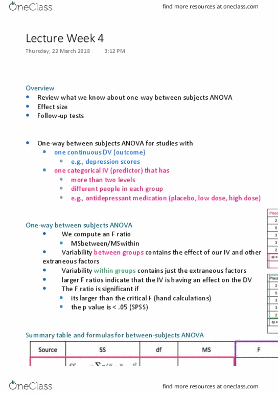
One-Way Repeated Measures ANOVA
A researcher is interested in looking at how alcohol consumption (IV) influences
attractiveness (DV)
-
Participants are rated on attractiveness on three different occasions. When having
consumed:
No alcohol
○
A low dose of alcohol
○
A high dose of alcohol
○
-
What type of follow-up tests should I do?
!Planned before looking at the data (a prior)
!Orthogonal contrasts
!Can use a decision wise alpha of .05 because each contrast is statistically
independent from the other contrasts - DON’T NEED FAMILYWISE ERROR
!Nonorthogonal contrasts or pairwise comparisons - singling out one more than
once eg, A vs B, A vs C
!Bonferroni correction to control familywise error
!adjusts p value based on number of tests
!Unplanned (post hoc)
!Tukey's HSD
!If we have the same number of people in each condition (equal ns)
!Controls familywise error by calculating the difference needed for an
honestly significant difference
! Scheffeì
!Most conservative/cautious method of controlling familywise error
!Uses a more stringent critical F from the overall ANOVA to evaluate
each comparison
Back to our example
!Let's say our researcher had planned to look at all pairwise comparisons
!No alcohol vs. low dose
!No alcohol vs. high dose
!Low dose vs. high dose
!We can ask SPSS for pairwise comparisons with a Bonferroni c
Putting it all together
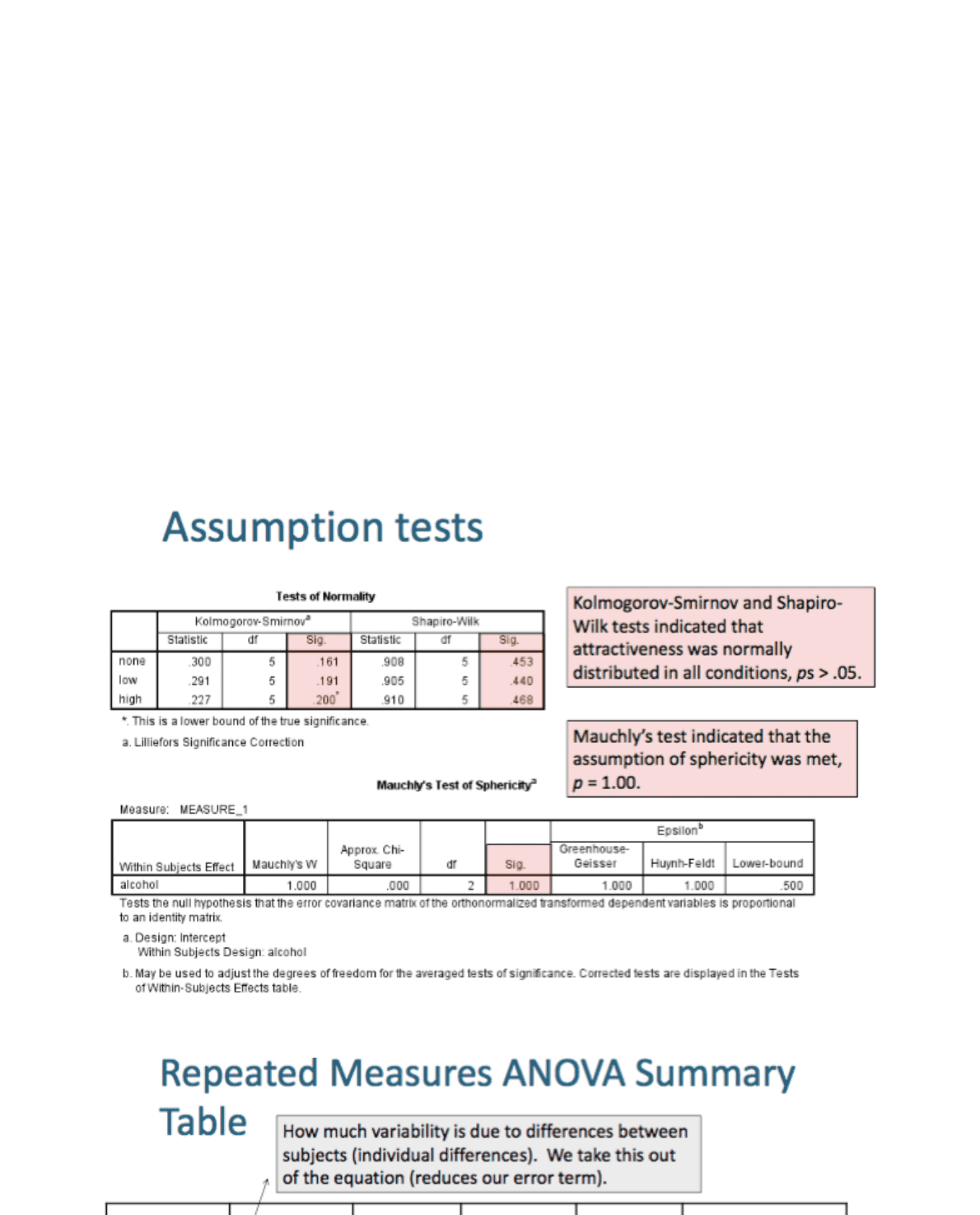
!All assumptions for the one-way repeated measures ANOVA were met.
!Attractiveness (DV) was measured on an interval scale.
!Kolmogorov-Smirnov and Shapiro-Wilk tests indicated that
attractiveness was normally distributed in all conditions, ps > .05.
!Mauchly's test indicated that the assumption of sphericity was met, p =
1.00.
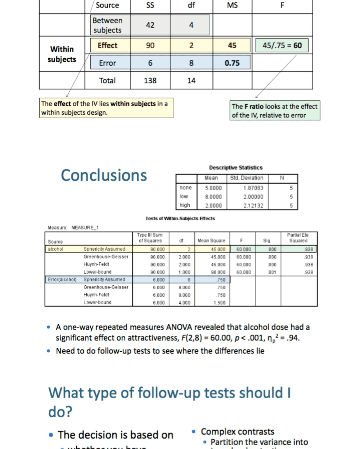
!A one-way repeated measures ANOVA revealed that alcohol dose had a
significant effect on
attractiveness, F(2,8) = 60.00, p < .001, ηp2 = .94.
• Bonferroni pairwise comparisons were conducted to compare each pair of conditions.
Participants were seen as significantly more attractive when they had consumed a
low dose of alcohol (M = 8.00, SD = 2.00) compared to no alcohol (M = 5.00, SD =
1.87), p = .016, and compared to a high dose of alcohol (M = 2.00, SD = 2.12), p
= .001.
•
Participants were seen as significantly less attractive when they had consumed a
high dose of alcohol compared to no alcohol, p = .016.
•
New example
!A researcher is interested in looking at how facial expression recognition
performance differs between four different emotional categories: Neutral, Happy,
Sad, and Angry.
!The dependent variable is mean expression recognition accuracy.
!Hypotheses
Neutral expressions will be recognised less accurately than
emotional expressions
§
Happy expressions will be recognised more accurately than negative
expressions
§
Angry expressions will be recognised more accurately than sad
expressions
§
What type of follow-up tests should I
do?
!The decision is based on
!whether you have specific hypotheses planned in advance - YES
!Hypotheses
!Neutral expressions will be recognised less accurately than emotional
expressions
!Happy expressions will be recognised more accurately than negative
expressions
!Angry expressions will be recognised more accurately than sad
expressions
!Are these contrasts or pairwise comparisons?
!Contrasts because some involve lumping conditions together
!Emotional expressions = happy, sad, angry
!Negative expressions = angry, sad
!Need to check if they are orthogonal
Orthogonal Contrasts
!For a group of contrasts to be orthogonal the following rules must be met:
!We compare two chunks of information per contrast
!We can leave groups out by assigning a weight of 0
!One chunk has positive coefficients, one chunk has negative coefficients
!The weights assigned to the group(s) in one chunk should be equal to the
number of groups in the other chunk
!The sum of the coefficients for a contrast should equal zero
!If a group is singled out in one contrast, it must be excluded
from any subsequent contrasts
!The number of contrasts should be equal to the dfeffect
!Number of conditions-1
Putting it all together
Most of the assumptions for the one-way repeated measures ANOVA were met.
!Emotion recognition accuracy (DV) was measured on a ratio scale.
!Kolmogorov-Smirnov and Shapiro-Wilk tests indicated that recognition
accuracy was normally distributed in the neutral, sad, and angry conditions,
ps > .05. Recognition accuracy was not normally distributed in happy condition
according to these normality tests, ps < .05. An examination of skew and kurtosis
statistics also revealed significant skew and kurtosis, ps < .05. However, ANOVA is
robust to violations of normality when there are more than 30 people in each
condition, so we proceeded with caution.
!Mauchly's test indicated that the assumption of sphericity was met, p = .807.
A one-way repeated measures ANOVA revealed that emotion category had a significant
effect on expression recognition accuracy, F(3,102) = 61.59, p < .001, ηp2 = .64.
• Orthogonal contrasts were conducted to test the specific hypotheses.
As predicted, neutral expressions were recognised significantly less accurately than
emotional expressions, F(1, 34) = 115.52, p < .001, ηp2 = .77.
•
As predicted, happy expressions were recognised significantly more accurately
than negative expressions, F(1, 34) = 37.58, p < .001, ηp2 = .53.
•
Contrary to predictions, angry expressions were recognised significantly less
accurately than sad expressions, F(1, 34) = 22.11, p < .001, ηp2 = .39.
•
When Assumptions are Violated
!ANOVA is robust to violations of normality when sample size is large (>30),
however when the sample size is small and the assumption is violated, we can use
a non-parametric equivalent.
!We'll learn these in week 10
!If the assumption of sphericity is violated, there are corrections
you can use.
!The corrections involve adjusting the df, which can affect the p value
!Greenhouse-Geisser (GG) is more conservative than Huynh-Feldt
(HF)
!Epsilon gives you an estimate of sphericity (1 is perfect)
!Use HF correction when sphericity is > .75
!Use GG correction when sphericity is unknown or < .75
If your DV is not measured on an interval or ratio scale, there are other tests you
can use
e.g., chi square – week 9
Assumption check
want to be not
significant so greater
than .05! Mean we
meet the normality
check
As we met the first
assumption above
we can look at the
sphericity assumed
The little p stands for partial
Werid n stands for Eta
Sigleing out one group more than once
above +1.96 or -1.96. both numbers are
significant so have to justify that the
study has more than 30 so proceed with
caution
Want to be
nonsignifiant
As Mauchly test was
met assumptions
above we can use
sphericity assumed
Week 7
Friday, 27 April 2018
11:53 AM

One-Way Repeated Measures ANOVA
A researcher is interested in looking at how alcohol consumption (IV) influences
attractiveness (DV)
-
Participants are rated on attractiveness on three different occasions. When having
consumed:
No alcohol
○
A low dose of alcohol
○
A high dose of alcohol
○
-
What type of follow-up tests should I do?
!Planned before looking at the data (a prior)
!Orthogonal contrasts
!Can use a decision wise alpha of .05 because each contrast is statistically
independent from the other contrasts - DON’T NEED FAMILYWISE ERROR
!Nonorthogonal contrasts or pairwise comparisons - singling out one more than
once eg, A vs B, A vs C
!Bonferroni correction to control familywise error
!adjusts p value based on number of tests
!Unplanned (post hoc)
!Tukey's HSD
!If we have the same number of people in each condition (equal ns)
!Controls familywise error by calculating the difference needed for an
honestly significant difference
! Scheffeì
!Most conservative/cautious method of controlling familywise error
!Uses a more stringent critical F from the overall ANOVA to evaluate
each comparison
Back to our example
!Let's say our researcher had planned to look at all pairwise comparisons
!No alcohol vs. low dose
!No alcohol vs. high dose
!Low dose vs. high dose
!We can ask SPSS for pairwise comparisons with a Bonferroni c
Putting it all together
!All assumptions for the one-way repeated measures ANOVA were met.
!Attractiveness (DV) was measured on an interval scale.
!Kolmogorov-Smirnov and Shapiro-Wilk tests indicated that
attractiveness was normally distributed in all conditions, ps > .05.
!Mauchly's test indicated that the assumption of sphericity was met, p =
1.00.
!A one-way repeated measures ANOVA revealed that alcohol dose had a
significant effect on
attractiveness, F(2,8) = 60.00, p < .001, ηp2 = .94.
• Bonferroni pairwise comparisons were conducted to compare each pair of conditions.
Participants were seen as significantly more attractive when they had consumed a
low dose of alcohol (M = 8.00, SD = 2.00) compared to no alcohol (M = 5.00, SD =
1.87), p = .016, and compared to a high dose of alcohol (M = 2.00, SD = 2.12), p
= .001.
•
Participants were seen as significantly less attractive when they had consumed a
high dose of alcohol compared to no alcohol, p = .016.
•
New example
!A researcher is interested in looking at how facial expression recognition
performance differs between four different emotional categories: Neutral, Happy,
Sad, and Angry.
!The dependent variable is mean expression recognition accuracy.
!Hypotheses
Neutral expressions will be recognised less accurately than
emotional expressions
§
Happy expressions will be recognised more accurately than negative
expressions
§
Angry expressions will be recognised more accurately than sad
expressions
§
What type of follow-up tests should I
do?
!The decision is based on
!whether you have specific hypotheses planned in advance - YES
!Hypotheses
!Neutral expressions will be recognised less accurately than emotional
expressions
!Happy expressions will be recognised more accurately than negative
expressions
!Angry expressions will be recognised more accurately than sad
expressions
!Are these contrasts or pairwise comparisons?
!Contrasts because some involve lumping conditions together
!Emotional expressions = happy, sad, angry
!Negative expressions = angry, sad
!Need to check if they are orthogonal
Orthogonal Contrasts
!For a group of contrasts to be orthogonal the following rules must be met:
!We compare two chunks of information per contrast
!We can leave groups out by assigning a weight of 0
!One chunk has positive coefficients, one chunk has negative coefficients
!The weights assigned to the group(s) in one chunk should be equal to the
number of groups in the other chunk
!The sum of the coefficients for a contrast should equal zero
!If a group is singled out in one contrast, it must be excluded
from any subsequent contrasts
!The number of contrasts should be equal to the dfeffect
!Number of conditions-1
Putting it all together
Most of the assumptions for the one-way repeated measures ANOVA were met.
!Emotion recognition accuracy (DV) was measured on a ratio scale.
!Kolmogorov-Smirnov and Shapiro-Wilk tests indicated that recognition
accuracy was normally distributed in the neutral, sad, and angry conditions,
ps > .05. Recognition accuracy was not normally distributed in happy condition
according to these normality tests, ps < .05. An examination of skew and kurtosis
statistics also revealed significant skew and kurtosis, ps < .05. However, ANOVA is
robust to violations of normality when there are more than 30 people in each
condition, so we proceeded with caution.
!Mauchly's test indicated that the assumption of sphericity was met, p = .807.
A one-way repeated measures ANOVA revealed that emotion category had a significant
effect on expression recognition accuracy, F(3,102) = 61.59, p < .001, ηp2 = .64.
• Orthogonal contrasts were conducted to test the specific hypotheses.
As predicted, neutral expressions were recognised significantly less accurately than
emotional expressions, F(1, 34) = 115.52, p < .001, ηp2 = .77.
•
As predicted, happy expressions were recognised significantly more accurately
than negative expressions, F(1, 34) = 37.58, p < .001, ηp2 = .53.
•
Contrary to predictions, angry expressions were recognised significantly less
accurately than sad expressions, F(1, 34) = 22.11, p < .001, ηp2 = .39.
•
When Assumptions are Violated
!ANOVA is robust to violations of normality when sample size is large (>30),
however when the sample size is small and the assumption is violated, we can use
a non-parametric equivalent.
!We'll learn these in week 10
!If the assumption of sphericity is violated, there are corrections
you can use.
!The corrections involve adjusting the df, which can affect the p value
!Greenhouse-Geisser (GG) is more conservative than Huynh-Feldt
(HF)
!Epsilon gives you an estimate of sphericity (1 is perfect)
!Use HF correction when sphericity is > .75
!Use GG correction when sphericity is unknown or < .75
If your DV is not measured on an interval or ratio scale, there are other tests you
can use
e.g., chi square – week 9
Assumption check
want to be not
significant so greater
than .05! Mean we
meet the normality
check
As we met the first
assumption above
we can look at the
sphericity assumed
The little p stands for partial
Werid n stands for Eta
Sigleing out one group more than once
above +1.96 or -1.96. both numbers are
significant so have to justify that the
study has more than 30 so proceed with
caution
Want to be
nonsignifiant
As Mauchly test was
met assumptions
above we can use
sphericity assumed
Week 7
Friday, 27 April 2018
11:53 AM
One-Way Repeated Measures ANOVA
A researcher is interested in looking at how alcohol consumption (IV) influences
attractiveness (DV)
-
Participants are rated on attractiveness on three different occasions. When having
consumed:
No alcohol
○
A low dose of alcohol
○
A high dose of alcohol
○
-
What type of follow-up tests should I do?
!Planned before looking at the data (a prior)
!Orthogonal contrasts
!Can use a decision wise alpha of .05 because each contrast is statistically
independent from the other contrasts - DON’T NEED FAMILYWISE ERROR
!Nonorthogonal contrasts or pairwise comparisons - singling out one more than
once eg, A vs B, A vs C
!Bonferroni correction to control familywise error
!adjusts p value based on number of tests
!Unplanned (post hoc)
!Tukey's HSD
!If we have the same number of people in each condition (equal ns)
!Controls familywise error by calculating the difference needed for an
honestly significant difference
! Scheffeì
!Most conservative/cautious method of controlling familywise error
!Uses a more stringent critical F from the overall ANOVA to evaluate
each comparison
Back to our example
!Let's say our researcher had planned to look at all pairwise comparisons
!No alcohol vs. low dose
!No alcohol vs. high dose
!Low dose vs. high dose
!We can ask SPSS for pairwise comparisons with a Bonferroni c
Putting it all together
!All assumptions for the one-way repeated measures ANOVA were met.
!Attractiveness (DV) was measured on an interval scale.
!Kolmogorov-Smirnov and Shapiro-Wilk tests indicated that
attractiveness was normally distributed in all conditions, ps > .05.
!Mauchly's test indicated that the assumption of sphericity was met, p =
1.00.
!A one-way repeated measures ANOVA revealed that alcohol dose had a
significant effect on
attractiveness, F(2,8) = 60.00, p < .001, ηp2 = .94.
• Bonferroni pairwise comparisons were conducted to compare each pair of conditions.
Participants were seen as significantly more attractive when they had consumed a
low dose of alcohol (M = 8.00, SD = 2.00) compared to no alcohol (M = 5.00, SD =
1.87), p = .016, and compared to a high dose of alcohol (M = 2.00, SD = 2.12), p
= .001.
•
Participants were seen as significantly less attractive when they had consumed a
high dose of alcohol compared to no alcohol, p = .016.
•
New example
!A researcher is interested in looking at how facial expression recognition
performance differs between four different emotional categories: Neutral, Happy,
Sad, and Angry.
!The dependent variable is mean expression recognition accuracy.
!Hypotheses
Neutral expressions will be recognised less accurately than
emotional expressions
§
Happy expressions will be recognised more accurately than negative
expressions
§
Angry expressions will be recognised more accurately than sad
expressions
§
What type of follow-up tests should I
do?
!The decision is based on
!whether you have specific hypotheses planned in advance - YES
!Hypotheses
!Neutral expressions will be recognised less accurately than emotional
expressions
!Happy expressions will be recognised more accurately than negative
expressions
!Angry expressions will be recognised more accurately than sad
expressions
!Are these contrasts or pairwise comparisons?
!Contrasts because some involve lumping conditions together
!Emotional expressions = happy, sad, angry
!Negative expressions = angry, sad
!Need to check if they are orthogonal
Orthogonal Contrasts
!For a group of contrasts to be orthogonal the following rules must be met:
!We compare two chunks of information per contrast
!We can leave groups out by assigning a weight of 0
!One chunk has positive coefficients, one chunk has negative coefficients
!The weights assigned to the group(s) in one chunk should be equal to the
number of groups in the other chunk
!The sum of the coefficients for a contrast should equal zero
!If a group is singled out in one contrast, it must be excluded
from any subsequent contrasts
!The number of contrasts should be equal to the dfeffect
!Number of conditions-1
Putting it all together
Most of the assumptions for the one-way repeated measures ANOVA were met.
!Emotion recognition accuracy (DV) was measured on a ratio scale.
!Kolmogorov-Smirnov and Shapiro-Wilk tests indicated that recognition
accuracy was normally distributed in the neutral, sad, and angry conditions,
ps > .05. Recognition accuracy was not normally distributed in happy condition
according to these normality tests, ps < .05. An examination of skew and kurtosis
statistics also revealed significant skew and kurtosis, ps < .05. However, ANOVA is
robust to violations of normality when there are more than 30 people in each
condition, so we proceeded with caution.
!Mauchly's test indicated that the assumption of sphericity was met, p = .807.
A one-way repeated measures ANOVA revealed that emotion category had a significant
effect on expression recognition accuracy, F(3,102) = 61.59, p < .001, ηp2 = .64.
• Orthogonal contrasts were conducted to test the specific hypotheses.
As predicted, neutral expressions were recognised significantly less accurately than
emotional expressions, F(1, 34) = 115.52, p < .001, ηp2 = .77.
•
As predicted, happy expressions were recognised significantly more accurately
than negative expressions, F(1, 34) = 37.58, p < .001, ηp2 = .53.
•
Contrary to predictions, angry expressions were recognised significantly less
accurately than sad expressions, F(1, 34) = 22.11, p < .001, ηp2 = .39.
•
When Assumptions are Violated
!ANOVA is robust to violations of normality when sample size is large (>30),
however when the sample size is small and the assumption is violated, we can use
a non-parametric equivalent.
!We'll learn these in week 10
!If the assumption of sphericity is violated, there are corrections
you can use.
!The corrections involve adjusting the df, which can affect the p value
!Greenhouse-Geisser (GG) is more conservative than Huynh-Feldt
(HF)
!Epsilon gives you an estimate of sphericity (1 is perfect)
!Use HF correction when sphericity is > .75
!Use GG correction when sphericity is unknown or < .75
If your DV is not measured on an interval or ratio scale, there are other tests you
can use
e.g., chi square – week 9
Assumption check
want to be not
significant so greater
than .05! Mean we
meet the normality
check
As we met the first
assumption above
we can look at the
sphericity assumed
The little p stands for partial
Werid n stands for Eta
Sigleing out one group more than once
above +1.96 or -1.96. both numbers are
significant so have to justify that the
study has more than 30 so proceed with
caution
Want to be
nonsignifiant
As Mauchly test was
met assumptions
above we can use
sphericity assumed
Week 7
Friday, 27 April 2018 11:53 AM
Document Summary
A researcher is interested in looking at how alcohol consumption (iv) influences attractiveness (dv) Participants are rated on attractiveness on three different occasions. Assumpti want to significan than . 05! meet the check nces having mption check t to be not ficant so greater. As we met th assumption we can look sphericity as. Werid n stand et the first tion above look at the ity assumed stands for partial tands for eta one. Planned before looking at the data (a prior) Can use a decision wise alpha of . 05 because each contrast is statistical independent from the other contrasts - don"t need familywise error. Nonorthogonal contrasts or pairwise comparisons - singling out one more th once eg, a vs b, a vs c. Adjusts p value based on number of tests. If we have the same number of people in each condition (equal n(cid:0)s) Controls familywise error by calculating the difference needed for an honestly significant difference.