1303AFE Lecture Notes - Lecture 7: Fiscal Policy, Output Gap, Real Interest Rate

47 views10 pages

harlequingnat161

30 May 2018

School

Griffith University

Department

Economics & Econometrics

Course

1303AFE

Professor

n/a

For unlimited access to Class Notes, a Class+ subscription is required.

Economics for Decision Making Week 7 Lecture Notes

AD-AS Model

• Aggregate demand- aggregate supply model

• Revise Demand and supply model

• Demand and supply (micro)→ AD-AS (macro)

Aggregate supply

• AS is the relationship between the quantity of real GDP supplied and the price level

when all other influences on production plans remain the same (ceteris paribus)

• Other things remaining the same,

o When the price level rises, the quantity of real GDP supplied increases

(increase P, Increase Ys)

• Along the AS curve, the only influence on production plans that changes is the P (P

→Ys: shown as movement along)

• All the other influences on production plan remain constant. Among these other

influences are:

o The money wage rate (nominal wage rate) (W)

o The money prices of other resources (e.g. if producing ice-cream then the

price of inputs like sugar or ice, oil price)

Potential GDP Line (LRAs- Long run aggregate supply)

• In AD-AS model, we have a perfectly vertical potential GDP Line drawn and fixed at

the full emp level of output (YFE)

o i.e. change in the price level does not influence the location of the line (YFE)

• the line can also be referred to as the long-run AS [LRAS] curve

Aggregate supply

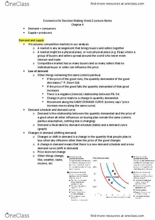
• Figure shows the aggregate schedule and aggregate supply curve

1. Potential GDP is $1.6 trillion and when P= 105, real GDP= potential GDP

2. If P> 105, real GDP> Potential GDP

3. If the P < 105, real GDP< potential GDP

find more resources at oneclass.com

Unlock document

This preview shows pages 1-3 of the document.
Unlock all 10 pages and 3 million more documents.

Already have an account? Log in

• Why the AS curve slopes upward

• If increase P and W is constant, the real wage rate (W/P) decrease falls and emp

increase as it is cheaper to hire workers. The qty of real GDP supplied increases

(increase Ys)

• For the economy as a whole, emp and real GDP change. 3 ways in which these

changes occur are

o Firms change their output rate

o Firms shut down temporarily or restart production

o Firms go out of business or start up in business

• Changes/ shift in AS

• AS shifts when any influence on production plans other than the price level changes

(P=0)

• In particular, aggregate supply shifts when:

o Potential GDP (Y*). So Y*→ AS

o W→ AS

o the money prices of other resources change (P of other resources → AS)

Y*→ AS

• Point C at the intersection of the potential GDP line and AS curve is an anchor point

1.An increase in potential GDP shifts the

potential GDP line rightward and

2. the aggregate supply curve shift rightward

from AS0 to AS1

find more resources at oneclass.com

Unlock document

This preview shows pages 1-3 of the document.
Unlock all 10 pages and 3 million more documents.

Already have an account? Log in

W→ AS

• A Change in the money (nominal) wage rate changes aggregate supply because it

chaged fir’s costs

• The higher the oey wage rate, the higher are fir’s costs ad the saller is the

quantity that firms are willing to supply at each price level

P of the other resources (Ex: change in oil price)→ AS

• A change in the money prices of other resources changes aggregate supply because

it chages fir’s costs

• The higher the oey prices of other resources, the higher are fir’s costs ad the

smaller is the quantity that firms are willing to supply at each price level

• So, an increase in the money prices of other resources (Ex: oil price increases) will

decrease (SHIFT LEFT) aggregate supply; vice versa

Aggregate demand

• AD is the relationship between the quantity of real GDP demanded and the price

level when all other influences on expenditure plans remain the same

• Other thing remaining the same,

o When the price level rises, the quantity of real GDP demanded decreases

(increase P, Decrease YD)

o When the price level falls, the quantity of real GDP demanded increases

(Decrease P, Increase YD)

• Figure shows the aggregate demand schedule and aggregate demand curve

find more resources at oneclass.com

Unlock document

This preview shows pages 1-3 of the document.
Unlock all 10 pages and 3 million more documents.

Already have an account? Log in

Document Summary

Economics for decision making week 7 lecture notes. Ad-as model: aggregate demand- aggregate supply model, revise demand and supply model, demand and supply (micro) ad-as (macro) Ys: shown as movement along: all the other influences on production plan remain constant. Among these other influences are: the money wage rate (nominal wage rate) (w, the money prices of other resources (e. g. if producing ice-cream then the price of inputs like sugar or ice, oil price) Potential gdp line (lras- long run aggregate supply) If increase p and w is constant, the real wage rate (w/p) decrease falls and emp increase as it is cheaper to hire workers. The qty of real gdp supplied increases (increase ys: for the economy as a whole, emp and real gdp change. In particular, aggregate supply shifts when: potential gdp (y*). So y* as: w as, the money prices of other resources change ( p of other resources as)

Related Questions

A. A decrease in aggregate supply can result in:

a recession
cost-push inflation
demand-pull inflation
unemployment

B. In the short run (intermediate-range) of the aggregate supply curve, higher aggregate demand will increase

the price level but reduce real GDP.
real GDP without raising the price level
the price level without affecting real GDP
both the price level and real GDP

C. Which of the following helps explain why real GDP is inversely related to the price level within the framework of the AD-AS model?

As prices fall, domestic consumers have an incentive to buy more of the cheaper goods and services
As prices fall, the wealth of people holding the fixed quantity of money increases, causing them to expand their purchases of goods and services
As prices fall, the government will have to reduce taxes, which will lead to an increase in the number of goods and services purchased
As prices fall, the monetary authorities will have to increase the money supply, which will lead to an increase in the number of goods and services purchased

carminewasp285

Part 1

Evaluate whether each of the following statements is true or false. Explain your answer and provide a supporting rationale.

a.The short-run aggregate supply (SAS) curve slopes upward because households spend more as their incomes increase.

b.The long-run aggregate supply curve can never shift.

c.Either a decrease in the nominal money supply by the Federal Reserve, all else held constant or an increase in the price level, all else held constant, will shift the aggregate demand (AD) curve to the left.

d.The Keynesian portion of the short-run aggregate supply (SAS) curve would be relevant during a recessionary situation.

e.Stagflation occurs when the aggregate demand (AD) curve shifts out on the upward sloping portion of the short-run aggregate supply (SAS) curve.

Part 2

Evaluate whether each of the following statements is true or false. Explain your answer and provide a supporting rationale, using graphs to support your answer. You can create graphs by hand and take pictures and upload them with your answers, or you may use Word or Excel, and upload the file created by these software packages.

a.If the real money demand is greater than the real money supply, interest rates must rise to reach equilibrium in the money market as institutions sell bonds to obtain more money.

b.The federal government's control of the money supply, which influences interest rates, is the primary tool that policymakers use to impact the macroeconomy.

c.A decrease in the reserve requirement decreases the money supply because banks have fewer reserves.

d.The real money demand curve shows how households and businesses change their spending in response to changes in the interest rate.

e.Both an increase in the nominal money supply by the Federal Reserve and an increase in the price level will cause the real money supply curve to shift to the right.

yellowseal739

In the Keynesian model

aggregate demand determines real GDP per year.

the short-run aggregate supply curve determines real GDP.

unemployment cannot persist for long periods of time.

the aggregate demand curve determines the price level.

A terrible winter storm causes enormous problems in the

northeastern

part of the United States. This would cause

the short-run aggregate supply curve to shift to the left, but would have no effect on the long-run aggregate supply curve.

both the short-run and the long-run aggregate supply curves to shift to the left, but the long-run aggregate supply curve would shift more than the short-run curve.

the short-run aggregate supply curve to shift to the left, and the long-run aggregate supply curve would shift to the right.

both the short-run and the long-run aggregate supply curves to shift to the right in equal amounts.

Equilibrium real GDP rises after the dollar strengthened. From this we can conclude that

the increase in aggregate demand was greater than the decrease in aggregate supply.

the decrease in aggregate demand was more than the increase in aggregate supply.

the decrease in aggregate demand was less than the increase in aggregate supply.

the increase in aggregate demand was less than the decrease in aggregate supply.

Saving is

the difference between real GDP and disposable income while savings is the difference between disposable income and consumption spending.

the amount one does not consume in a given period of time while savings is the accumulation of past periods of saving.

the difference between disposable income and spending on goods and serviceswhile savings is the difference between real GDP and disposable income.

the accumulation of past periods of savings while savings is the amount of disposable income that is not consumed in a given period of time.

A permanent reduction in investment spending leads to

a proportional decrease in real GDP.

a more than proportional decrease in real GDP.

a more than proportional increase in real GDP.

a less than proportional decrease in real GDP.

An increase in net exports leads to an increase in real GDP. Further,

consumption spending increases while investment spending decreases.

consumption spending increases but saving does not change.

consumption spending and saving increase.

government spending decreases to offset the increase in net exports.

An increase in aggregate spending that is caused by a factor other than the price level will lead to the

aggregate demand curve shifting to the right.

aggregate supply curve shifting to the right.

aggregate supply curve shifting to the left.

aggregate demand curve shifting to the left.

The marginal propensity to consume is 0.9. The multiplier is

0.9.

1.11.

0.1.

10.

When the SRAS curve slopes upward, the actual affect of an increase in real autonomous spending on equilibrium real GDP is smaller than predicted by the multiplier because

real GDP increases.

the price level rises

the price level falls.

real GDP decreases.

Other things equal, the lower the total real value of final goods and services demanded in the economy the

more the production possibilities cure shifts to the left.

lower the price level.

higher the price level.

lower the level of endowments.

The long-run aggregate supply curve can be thought of as the

level of output for which real GDP equals nominal GDP.

level of output that the nation is currently producing.

level of real GDP associated with a constant price level.

full-employment level of real GDP.

1303AFE Lecture Notes - Lecture 7: Fiscal Policy, Output Gap, Real Interest Rate

Document Summary

Get access

Related Documents

1303AFE Lecture Notes - Lecture 2: Shortage, Economic Equilibrium, Price Ceiling

ECON 1010 Study Guide - Aggregate Demand, Aggregate Supply, Gdp Deflator

EC140 Chapter Notes - Chapter 26: Monetarism, Exchange Rate, Output Gap

Related Questions