MARK3054 Lecture Notes - Lecture 8: Arbitrage, Demand Curve, Price Discrimination


Topic 8: Pricing: Demand Curve and Revenue Management
Demand Curves:
1. Linear Q= a-bp (Q and b will change, i.e. elasticity changes with price)
2. Power Q=Apb (elasticity stays constant as price changes)
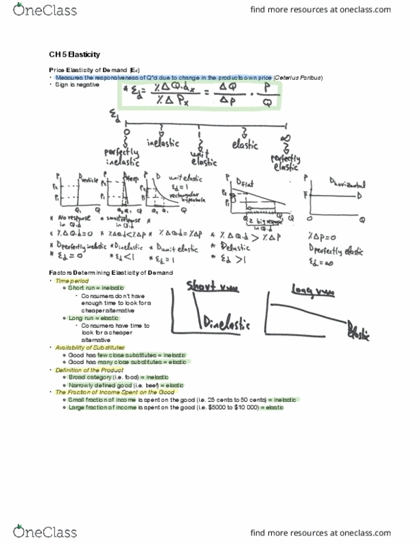
Elasticity= fraction change in demand/fraction change in price
E=1 (unit elasticity)
E>1 (decrease price of product, will increase revenue i.e. elastic)
E<1 (decrease price of product, will decrease revenue i.e. inelastic)
Consumers may make inferences of price changes:
-new model about to be released
-product is not selling well
-quality has decreased
-price will come down further, so wait
OR
-product is popular and may soon be unavailable
-very good value
-more price increases may be ahead
Using Solver to optimise price:
1. Find demand curve
2. Setup profit function based on demand curve
3. Maximise profit based on constraints (prices are non-negative, prices follow in a range,
inventory limit)
Price Competition:
Going-rate (homogenous commodities)
Competitive bidding (compete with unknown number of suppliers with no knowledge of their prices)
Differential Pricing:
Price Discrimination:
1st Degree (charge customers exactly what they are willing to pay i.e. tenders)
2nd degree (wholesale, retail, different prices depending on quantity, bulk buying)
3rd degree (divide customers into segments, charging different prices to different segments i.e.
product or service differentiation)
1st degree price discrimination is hard: typically monopoly seller, identify reservation prices, prevent
potential arbitrage, customers may view as unfair.
find more resources at oneclass.com
find more resources at oneclass.com
Document Summary
Topic 8: pricing: demand curve and revenue management. Demand curves: linear q= a-bp (q and b will change, i. e. elasticity changes with price, power q=apb (elasticity stays constant as price changes) Elasticity= fraction change in demand/fraction change in price. E>1 (decrease price of product, will increase revenue i. e. elastic) E<1 (decrease price of product, will decrease revenue i. e. inelastic) Product is popular and may soon be unavailable. Using solver to optimise price: find demand curve, setup profit function based on demand curve, maximise profit based on constraints (prices are non-negative, prices follow in a range, inventory limit) Competitive bidding (compete with unknown number of suppliers with no knowledge of their prices) 1st degree (charge customers exactly what they are willing to pay i. e. tenders) 2nd degree (wholesale, retail, different prices depending on quantity, bulk buying) 3rd degree (divide customers into segments, charging different prices to different segments i. e. product or service differentiation)