BIOL 4150 Lecture Notes - Lecture 9: Population Viability Analysis, Exponential Decay, Mortality Rate

2 May 2018
School
Department
Course
Professor

Chapter 9
dV/dt = growth -mortality due to consumption
(prey)
•
dN/dt = growth due to consumption -mortality
(predator)
•
Generalized Lotka-Volterra model
Functional and numerical responses
•
Plant growth in relation to rainfall
•
Consumer-resource dynamics
•
Population viability analysis
•
Kangaroo-plant dynamics:
Put kangaroos in small paddocks and let them
deplete plant biomass over time
•
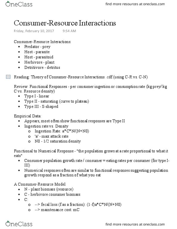
Recorded bite rate and bite size per unit foraging
time
•
c=81.172
○
b=-0.012
○
e^0 = 1 --> exponential decay,
starts at c
□
1-e^x --> starts at 0, decays as it
approaches max value (=c)
□
If b increases, curve becomes
more steep
□
All curves in this function…
!
I(V)=c*(1-e^(b*V)) (..)=decay term *this is
the functional response
○
*growth rate is compromised with low
vegetation biomass
Consumption rate increases and then plateaus with
increasing vegetation biomass
•
Functional response:
Count kangaroos and measure plant biomass every 3
years
•
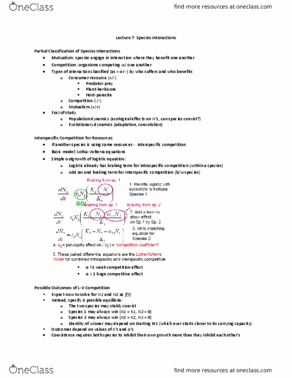
Calculate per capita growth rate (=numerical
response) for each pair of censuses
•
Reached carrying capacity
○
Plant cycle droughts
○
Predation
○
Immigration
○
Doesn't mean that vegetation is at
equilibrium point
*dotted line = vegetation that
supports kangaroo population (not
too little or too much)
Growth becomes and stays negative due
to lag in response (losing more
individuals over time; takes a while for
population to decline)
*apex --> when growth rate = 0
Possible explanations for graphs:
•
Growth rate decreases as available vegetation
decreases because they don't have enough energy to
survive and reproduce in the same manner
•
*determined by regression
!
a = 0.5 (max rate of decrease (how death is
affected by food); constant)
○
Magnitude dictates how fast curve
changes
!
Carrying capacity of kangaroos
will be at lower plant biomass
□
Curve will be sharper if individual is a
more efficient feeder
!
f= -0.007 (slope; decay for curve)
○
d=0.4 (estimate of death)
○
Per capita rate of increase vs. plant
biomass
!
r(V) = a(1-e^(f*V)) - d
○
Maximum rate of increase: rm = c -a = 0.5 -0.4 =
0.1
•
Minimum rate of growth (when biomass = 0) = d
•
Numerical response:
Record above ground plant biomass every 3 months
in exclosures
•
Positively related to rainfall
•
Negatively related to plant biomass
•
Highest growth at low biomass
•
Delta(V,R) = -55.12 -0.01535V -0.00056V^2
+ 2.5*R
○
Plant growth and biomass are highest with
more rainfall (parabola is wider)
○
V(0) = 30
!
dV/dt (t) = Delta(V(t),R(t)) -N(t)*I(V(t))
○
N(0) = 0.1
!
dN/dt (t) = N(t)*(r(V(t)))
○
Plant growth vs. plant biomass (upside down
parabola)
•
dV/dt >0
◊
Biomass increases below
line (growth>consumption)
!
dV/dt <0
◊
Biomass decreases above
line (consumption>growth)
!
Plant zero isocline decreases
□
iso1(V)=(Delta(V,R)) / I(V)
!
dV/dt=0 when N=(Delta(V,R)) / I(V)
○
Density decreases if left to
line (die)
!
Density increases if right to
line (thrives)
!
Kangaroo zero isocline is linear at
V = 220
□
iso2=(1/f)*ln(1-(d/a))
!
dN/dt=0 when r(V)=0
○
Carrying capacity when taking both
factors into consideration
!
Max growth rate at low
density
!
Carrying capacity when r=0
!
Growth rate (r) vs. Density (N)
□
If only considering kangaroos:
!
Looks like a convertible growth
rate vs. density used for the
kangaroos
□
--> density-dependence
□
If only considering vegetation:
!
Point of interception: when kangaroo density
and plant biomass are balanced
○
Numerical response -analogous
function that dictates the growth rate of
the consumer as a function of the
environment (V)
!
Note: functional response -how feeding rate is
influenced by environment (V)
○
Par(mfrow=c(2,2))
!
Yearmax<-20
!
Not yearly census
□
Tmax<-4*yearmax
!
Alpha<-55.12
!
Beta<-0.01535
!
Gamma<-0.00056
!
Phi<-2.50
!
D<-0.4
!
A<-0.5
!
F<-0.007
!
C<-86
!
B<-0.029
!
*rainfall
□
R<-numeric(tmax)
!
*tmax=timestamps, mean=60,
sdr=28
□
Rtemp<-rnorm(tmax,60,28)
!
*assigns rainfall with normal
distribution; max --> no negative
rainfall (don’t want values to the
left of the normal distribution)
□
If <0 will use 0
!
If >0 with use Rtemp at 't'
!
Max value of alternatives
□
For(i in 1:tmax)R[t]<-max(0,Rtemp[t])
!
Year<-numeric(tmax)
!
N<-numeric(tmax)
!
N[1]<-0.5
!
*sets up vectors
□
V[1]<-200
!
*quarterly basis
□
Year[1]<-0.25
!
For(t in 2:tmax{
!
Assign vegetation value from year
before + other aspects (like
growth rate)
□
Use max because it cant be <0
□
Use subtraction (if not use max
will have negative value)
□
Parabolic ?
□
N[t-1] …. <- functional response
= growth -consumption
□
V[t] = V[t-1] + growth -
consumption
□
V[t+1] will have highest
growth rate
!
Delta(V,R) = -55.12 -
…V - ….V^2 + 2.5R
◊
dV(t)/dt = Delta(V(t),R(t)) -
N(t)*I(V(t))
!
If V[t]=0,
□
V[t]<-max(0,V[t-1]+(alpha-beta*V[t-1]-
gamma*V[t-1]^2+phi*R[t-1)-
N[t-1]*c*(1-exp(-b*V[t-1])))
!
N[t] = N[t-1] + growth due to
consumption -mortality
□
N[t+1] =0 *will not recover
!
dN(t)/dt = N(t)*(r(V(t)))
!
If N[t] = 0,
□
N[t]<-max(0,N[t-1]+N[t-1]*(a*(1-exp(-
f*V[t-1]-d)))
!
Year[t]<-t/4
!
}
!
Rmax<-ceiling(max(R)*1.2)
!
Nmax<-ceiling(max(N)*1.2)
!
Vmax<-ceiling(max(V)*1.2)
!
Barplot(R,…….)
!
Plot(….)
!
Plot(…)
!
Stochastic Dynamics:
○
Life-history stages of kangaroo -->
dependence on vegetation
!
*note: lag between rainfall --> vegetation -->
kangaroo population
○
Stochastic but has signature with some
variation
!
Long recovery time when adjusting to
resources needed
!
Shows slower response to
environmental variation (recovery)
!
Must anticipate long recovery intervals
for management
!
-->quasi-cycle
○
Kangaroo density vs. vegetation biomass
•
Plant growth:
11/16/17
Populations track a stochastic moving target (in this
case, rainfall)
•
Bounded population growth stems from density-
dependent processes, so they are naturally regulated
•
4 ha: u = 16 years
○
10 ha: u=93 years
○
16 ha: u = 242 years
○
Population viability analysis of kangaroos:
extinction probability in reserves of different size
•
Longer time in low recovery stage
□
Incorporates stochastic variation in
resource --> lag
!
Interactive model: where rainfall, plants and
herbivores interact
○
Probability of persisting 100 years is higher in the
logistic model compared to the interactive model
with increasing area size
•
Centripetal Systems (quasi-cycle)
Hyperpredation on endemic prey induced by
invasion by an invulnerable alternate prey can cause
collapse to dangerously low levels
•
Ex. Endemic birds on a number of islands in the
southern Pacific Ocean have gone extinct following
the introduction of rabbits and cats
•
*see slide
○
dB(t)/dt = prey growth (recruitment) -
prey consumption (predation) *birds
!
dR(t)/dt = prey growth -prey
consumption *rabbits
!
dC(t)/dt = growth (recruitment) due to
consumption -mortality *cats
!
Differential Equations: instantaneous change
(process of depletion)
○
Model:
•
= Type I Functional Response * Prey
Preference
○
=(C(t)*uBB(t))*((alpha*B(t))/(R(t)+alpha*B(t)
))
○
= type 1 functional response
(linear)
□
Negative effect on prey
□
Positive effect on predator
□
Consumption rate: u*quantity of
birds*quantity of cats
!
uB= slope
○
Lambda = conversion coefficient
○
Prey Consumption:
•
Birds>rabbits when both equally
common
!
Preference increases with abundance of prey
○
If alpha = 1, there is no preference
(indiscriminate)
○
*consumption rate is mediated by the
preference of prey
○
= type 2 functional response (curved)
○
Alpha -dictates degree of preference
•
Max rate of increase by exotic prey: rmaxR =
2
○
Carrying capacity of endemic prey: KB=1000
○
Carrying capacity of exotic prey: KR=5000
○
Attack rate on endemic prey by predator: uB =
0.1
○
Attack rate on exotic prey by predator: uR =
0.1
○
Preference on endemic relative to exotic:
alpha=3
○
*currency of birds into new kittens
!
Conversion of attacked endemics into
predators: lambdaB=0.01
○
Conversion of attacked exotics into predator:
lamdaR = 0.01
○
Mortality rate of predators: v=0.5
○
End of simulation: T=50
○
Max rate of increase by endemic prey: rmaxB = 0.1
•
*see slide (cats = 0)
○
Bird population remains constant while rabbit
population increases to carrying capacity over
time
○
Therefore --> (1-
(B[t-1]+R[t-1])/K) in bird
equation
□
If equal competitors: include R[t-1] in N
!
If they both compete for the same resources,
must include exploitative competition
○
Endemic prey (birds) coexist with introduced prey
species (rabbits)
•
*see slide (rabbits =0)
○
Both populations fluctuate until they reach an
equilibrium
○
Endemic prey (birds) can also coexist with
introduced predators (cats)
•
Cat population grows due to large number of
prey available
○
Due to bird preference, predation would be
stronger on the bird population
○
In the presence of an exotic competitor however,
endemic birds crash and face extinction
•
Hyperpredation due to apparent competition and extinction
of endemic prey
11/21/17
rmaxB <-0.1/100
○
rmaxR<-2/100
○
KB<-1000
○
KR<-5000
○
uB<-0.1/100
○
uR<-0.1/100
○
alpha<-3
○
lambdaB<-0.01/100
○
lambdaR<-0.01/100
○
v<-0.5/100
○
T<-50
○
R<-numeric(5000)
○
B<-numeric(5000)
○
C<-numeric(5000)
○
R[1]<-20
○
B[1]<-20
○
C[1]<-20
○
For( t in 2:5000){
B[t]<-B[t-1] + rmaxB*B[t-1]*(1-B[t-1]/KB) -
C[t-1]*uB*B[t-1]*((alpha*B[t-1])/(R[t-1] +
alpha*B[t-1]))
R[t]<-...
C[t]<-…
}
○
Define parameters:
•
*see courselink for full r-coding
•
Modeling:
Endemic skunk
○
Exotic prey (feral pigs) were brought in
several decades ago before it was a reserve
○
Colonization coincided with decline of
the fox and increase in the skunk
populations
!
Golden eagles recently immigrated from the
mainland
○
6 endemic fox species, each on different islands in
the archipelago
•
Apparent and actual competition (skunks
increase while fox declines)
○
Direct interaction between fox and skunk
○
Eagle --> fox > pigs > skunks
○
Negative feedback on each population -->
limits on population size
○
*see interaction between fox, pig, skunk and eagle
•
rf*F(1 -(F + betafsS)/Kf) -uf(piF /(piF
+sigmaS +P)*EF
!
pi=preference
!
dF/dt = recruitment -competition -
consumption
○
Rs*S (1-(S+betasfF)/Ks) -us(sigmaS/
piF +sigmaS + P)*ES
!
dS/dt = recruitment -competition -
consumption
○
rp*P(1-P/Kp) -up(P/(piF + sigmaS +
P)) EP
!
dP/dt = recruitment -consumption
○
=(lambdaf*uf*piF^2 +
lambdas*us*sigmaS^2 +
lambdap*up*P^2)*E /piF+sigmaS + P -
vE
!
dE/dt = recruitment due to consumption -
mortality
○
Modeling:
•
Eagles and skunks go extinct while fox
population recovers
○
Eagles can get enough energy to survive
○
Skunk population declines due to competition
with foxes (out competed)
○
Without pigs:
•
All populations persist
○
Eagle population --> logistic growth
○
Pig --> highest conversion coefficient
○
--> apparent competition
!
Foxes have the lowest density
○
Pigs are able to tip the balance so system does
not become overwhelmed
○
With all prey:
•
Just pigs --> eagles will hunt more skunks and
foxes
○
Just eagles --> pig populations will cause
eagles to move back to island from mainland
○
Must eradicate pigs and eagles at the same time
•
Ex. Channel Islands
*must adjust
parameters
(yearly vs.
year/100)
--> all time-
dependent
parameters must
be modified by
/100
Consumer-Resource Dynamics
Tuesday,+ November+ 14,+2017
11:32+AM

Chapter 9
dV/dt = growth -mortality due to consumption
(prey)
•
dN/dt = growth due to consumption -mortality
(predator)
•
Generalized Lotka-Volterra model
Functional and numerical responses
•
Plant growth in relation to rainfall
•
Consumer-resource dynamics
•
Population viability analysis
•
Kangaroo-plant dynamics:
Put kangaroos in small paddocks and let them
deplete plant biomass over time
•
Recorded bite rate and bite size per unit foraging
time
•
c=81.172
○
b=-0.012
○
e^0 = 1 --> exponential decay,
starts at c
□
1-e^x --> starts at 0, decays as it
approaches max value (=c)
□
If b increases, curve becomes
more steep
□
All curves in this function…
!
I(V)=c*(1-e^(b*V)) (..)=decay term *this is
the functional response
○
*growth rate is compromised with low
vegetation biomass
Consumption rate increases and then plateaus with
increasing vegetation biomass
•
Functional response:
Count kangaroos and measure plant biomass every 3
years
•
Calculate per capita growth rate (=numerical
response) for each pair of censuses
•
Reached carrying capacity
○
Plant cycle droughts
○
Predation
○
Immigration
○
Doesn't mean that vegetation is at
equilibrium point
*dotted line = vegetation that
supports kangaroo population (not
too little or too much)
Growth becomes and stays negative due
to lag in response (losing more
individuals over time; takes a while for
population to decline)
*apex --> when growth rate = 0
Possible explanations for graphs:
•
Growth rate decreases as available vegetation
decreases because they don't have enough energy to
survive and reproduce in the same manner
•
*determined by regression
!
a = 0.5 (max rate of decrease (how death is
affected by food); constant)
○
Magnitude dictates how fast curve
changes
!
Carrying capacity of kangaroos
will be at lower plant biomass
□
Curve will be sharper if individual is a
more efficient feeder
!
f= -0.007 (slope; decay for curve)
○
d=0.4 (estimate of death)
○
Per capita rate of increase vs. plant
biomass
!
r(V) = a(1-e^(f*V)) - d
○
Maximum rate of increase: rm = c -a = 0.5 -0.4 =
0.1
•
Minimum rate of growth (when biomass = 0) = d
•
Numerical response:
Record above ground plant biomass every 3 months
in exclosures
•
Positively related to rainfall
•
Negatively related to plant biomass
•
Highest growth at low biomass
•
Delta(V,R) = -55.12 -0.01535V -0.00056V^2
+ 2.5*R
○
Plant growth and biomass are highest with
more rainfall (parabola is wider)
○
V(0) = 30
!
dV/dt (t) = Delta(V(t),R(t)) -N(t)*I(V(t))
○
N(0) = 0.1
!
dN/dt (t) = N(t)*(r(V(t)))
○
Plant growth vs. plant biomass (upside down
parabola)
•
dV/dt >0
◊
Biomass increases below
line (growth>consumption)
!
dV/dt <0
◊
Biomass decreases above
line (consumption>growth)
!
Plant zero isocline decreases
□
iso1(V)=(Delta(V,R)) / I(V)
!
dV/dt=0 when N=(Delta(V,R)) / I(V)
○
Density decreases if left to
line (die)
!
Density increases if right to
line (thrives)
!
Kangaroo zero isocline is linear at
V = 220
□
iso2=(1/f)*ln(1-(d/a))
!
dN/dt=0 when r(V)=0
○
Carrying capacity when taking both
factors into consideration
!
Max growth rate at low
density
!
Carrying capacity when r=0
!
Growth rate (r) vs. Density (N)
□
If only considering kangaroos:
!
Looks like a convertible growth
rate vs. density used for the
kangaroos
□
--> density-dependence
□
If only considering vegetation:
!
Point of interception: when kangaroo density
and plant biomass are balanced
○
Numerical response -analogous
function that dictates the growth rate of
the consumer as a function of the
environment (V)
!
Note: functional response -how feeding rate is
influenced by environment (V)
○
Par(mfrow=c(2,2))
!
Yearmax<-20
!
Not yearly census
□
Tmax<-4*yearmax
!
Alpha<-55.12
!
Beta<-0.01535
!
Gamma<-0.00056
!
Phi<-2.50
!
D<-0.4
!
A<-0.5
!
F<-0.007
!
C<-86
!
B<-0.029
!
*rainfall
□
R<-numeric(tmax)
!
*tmax=timestamps, mean=60,
sdr=28
□
Rtemp<-rnorm(tmax,60,28)
!
*assigns rainfall with normal
distribution; max --> no negative
rainfall (don’t want values to the
left of the normal distribution)
□
If <0 will use 0
!
If >0 with use Rtemp at 't'
!
Max value of alternatives
□
For(i in 1:tmax)R[t]<-max(0,Rtemp[t])
!
Year<-numeric(tmax)
!
N<-numeric(tmax)
!
N[1]<-0.5
!
*sets up vectors
□
V[1]<-200
!
*quarterly basis
□
Year[1]<-0.25
!
For(t in 2:tmax{
!
Assign vegetation value from year
before + other aspects (like
growth rate)
□
Use max because it cant be <0
□
Use subtraction (if not use max
will have negative value)
□
Parabolic ?
□
N[t-1] …. <- functional response
= growth -consumption
□
V[t] = V[t-1] + growth -
consumption
□
V[t+1] will have highest
growth rate
!
Delta(V,R) = -55.12 -
…V - ….V^2 + 2.5R
◊
dV(t)/dt = Delta(V(t),R(t)) -
N(t)*I(V(t))
!
If V[t]=0,
□
V[t]<-max(0,V[t-1]+(alpha-beta*V[t-1]-
gamma*V[t-1]^2+phi*R[t-1)-
N[t-1]*c*(1-exp(-b*V[t-1])))
!
N[t] = N[t-1] + growth due to
consumption -mortality
□
N[t+1] =0 *will not recover
!
dN(t)/dt = N(t)*(r(V(t)))
!
If N[t] = 0,
□
N[t]<-max(0,N[t-1]+N[t-1]*(a*(1-exp(-
f*V[t-1]-d)))
!
Year[t]<-t/4
!
}
!
Rmax<-ceiling(max(R)*1.2)
!
Nmax<-ceiling(max(N)*1.2)
!
Vmax<-ceiling(max(V)*1.2)
!
Barplot(R,…….)
!
Plot(….)
!
Plot(…)
!
Stochastic Dynamics:
○
Life-history stages of kangaroo -->
dependence on vegetation
!
*note: lag between rainfall --> vegetation -->
kangaroo population
○
Stochastic but has signature with some
variation
!
Long recovery time when adjusting to
resources needed
!
Shows slower response to
environmental variation (recovery)
!
Must anticipate long recovery intervals
for management
!
-->quasi-cycle
○
Kangaroo density vs. vegetation biomass
•
Plant growth:
11/16/17
Populations track a stochastic moving target (in this
case, rainfall)
•
Bounded population growth stems from density-
dependent processes, so they are naturally regulated
•
4 ha: u = 16 years
○
10 ha: u=93 years
○
16 ha: u = 242 years
○
Population viability analysis of kangaroos:
extinction probability in reserves of different size
•
Longer time in low recovery stage
□
Incorporates stochastic variation in
resource --> lag
!
Interactive model: where rainfall, plants and
herbivores interact
○
Probability of persisting 100 years is higher in the
logistic model compared to the interactive model
with increasing area size
•
Centripetal Systems (quasi-cycle)
Hyperpredation on endemic prey induced by
invasion by an invulnerable alternate prey can cause
collapse to dangerously low levels
•
Ex. Endemic birds on a number of islands in the
southern Pacific Ocean have gone extinct following
the introduction of rabbits and cats
•
*see slide
○
dB(t)/dt = prey growth (recruitment) -
prey consumption (predation) *birds
!
dR(t)/dt = prey growth -prey
consumption *rabbits
!
dC(t)/dt = growth (recruitment) due to
consumption -mortality *cats
!
Differential Equations: instantaneous change
(process of depletion)
○
Model:
•
= Type I Functional Response * Prey
Preference
○
=(C(t)*uBB(t))*((alpha*B(t))/(R(t)+alpha*B(t)
))
○
= type 1 functional response
(linear)
□
Negative effect on prey
□
Positive effect on predator
□
Consumption rate: u*quantity of
birds*quantity of cats
!
uB= slope
○
Lambda = conversion coefficient
○
Prey Consumption:
•
Birds>rabbits when both equally
common
!
Preference increases with abundance of prey
○
If alpha = 1, there is no preference
(indiscriminate)
○
*consumption rate is mediated by the
preference of prey
○
= type 2 functional response (curved)
○
Alpha -dictates degree of preference
•
Max rate of increase by exotic prey: rmaxR =
2
○
Carrying capacity of endemic prey: KB=1000
○
Carrying capacity of exotic prey: KR=5000
○
Attack rate on endemic prey by predator: uB =
0.1
○
Attack rate on exotic prey by predator: uR =
0.1
○
Preference on endemic relative to exotic:
alpha=3
○
*currency of birds into new kittens
!
Conversion of attacked endemics into
predators: lambdaB=0.01
○
Conversion of attacked exotics into predator:
lamdaR = 0.01
○
Mortality rate of predators: v=0.5
○
End of simulation: T=50
○
Max rate of increase by endemic prey: rmaxB = 0.1
•
*see slide (cats = 0)
○
Bird population remains constant while rabbit
population increases to carrying capacity over
time
○
Therefore --> (1-
(B[t-1]+R[t-1])/K) in bird
equation
□
If equal competitors: include R[t-1] in N
!
If they both compete for the same resources,
must include exploitative competition
○
Endemic prey (birds) coexist with introduced prey
species (rabbits)
•
*see slide (rabbits =0)
○
Both populations fluctuate until they reach an
equilibrium
○
Endemic prey (birds) can also coexist with
introduced predators (cats)
•
Cat population grows due to large number of
prey available
○
Due to bird preference, predation would be
stronger on the bird population
○
In the presence of an exotic competitor however,
endemic birds crash and face extinction
•
Hyperpredation due to apparent competition and extinction
of endemic prey
11/21/17
rmaxB <-0.1/100
○
rmaxR<-2/100
○
KB<-1000
○
KR<-5000
○
uB<-0.1/100
○
uR<-0.1/100
○
alpha<-3
○
lambdaB<-0.01/100
○
lambdaR<-0.01/100
○
v<-0.5/100
○
T<-50
○
R<-numeric(5000)
○
B<-numeric(5000)
○
C<-numeric(5000)
○
R[1]<-20
○
B[1]<-20
○
C[1]<-20
○
For( t in 2:5000){
B[t]<-B[t-1] + rmaxB*B[t-1]*(1-B[t-1]/KB) -
C[t-1]*uB*B[t-1]*((alpha*B[t-1])/(R[t-1] +
alpha*B[t-1]))
R[t]<-...
C[t]<-…
}
○
Define parameters:
•
*see courselink for full r-coding
•
Modeling:
Endemic skunk
○
Exotic prey (feral pigs) were brought in
several decades ago before it was a reserve
○
Colonization coincided with decline of
the fox and increase in the skunk
populations
!
Golden eagles recently immigrated from the
mainland
○
6 endemic fox species, each on different islands in
the archipelago
•
Apparent and actual competition (skunks
increase while fox declines)
○
Direct interaction between fox and skunk
○
Eagle --> fox > pigs > skunks
○
Negative feedback on each population -->
limits on population size
○
*see interaction between fox, pig, skunk and eagle
•
rf*F(1 -(F + betafsS)/Kf) -uf(piF /(piF
+sigmaS +P)*EF
!
pi=preference
!
dF/dt = recruitment -competition -
consumption
○
Rs*S (1-(S+betasfF)/Ks) -us(sigmaS/
piF +sigmaS + P)*ES
!
dS/dt = recruitment -competition -
consumption
○
rp*P(1-P/Kp) -up(P/(piF + sigmaS +
P)) EP
!
dP/dt = recruitment -consumption
○
=(lambdaf*uf*piF^2 +
lambdas*us*sigmaS^2 +
lambdap*up*P^2)*E /piF+sigmaS + P -
vE
!
dE/dt = recruitment due to consumption -
mortality
○
Modeling:
•
Eagles and skunks go extinct while fox
population recovers
○
Eagles can get enough energy to survive
○
Skunk population declines due to competition
with foxes (out competed)
○
Without pigs:
•
All populations persist
○
Eagle population --> logistic growth
○
Pig --> highest conversion coefficient
○
--> apparent competition
!
Foxes have the lowest density
○
Pigs are able to tip the balance so system does
not become overwhelmed
○
With all prey:
•
Just pigs --> eagles will hunt more skunks and
foxes
○
Just eagles --> pig populations will cause
eagles to move back to island from mainland
○
Must eradicate pigs and eagles at the same time
•
Ex. Channel Islands
*must adjust
parameters
(yearly vs.
year/100)
--> all time-
dependent
parameters must
be modified by
/100
Consumer-Resource Dynamics
Tuesday,+ November+ 14,+2017 11:32+AM
Document Summary
Generalized lotka-volterra model dv/dt = growth - mortality due to consumption (prey) dn/dt = growth due to consumption - mortality (predator) Put kangaroos in small paddocks and let them deplete plant biomass over time. Recorded bite rate and bite size per unit foraging time. Consumption rate increases and then plateaus with increasing vegetation biomass c=81. 172 b=-0. 012. I(v)=c*(1- e^(b*v)) ()=decay term *this is the functional response. All curves in this function e^0 = 1 --> exponential decay, starts at c. 1-e^x --> starts at 0, decays as it approaches max value (=c) *growth rate is compromised with low vegetation biomass. Count kangaroos and measure plant biomass every 3 years. Calculate per capita growth rate (=numerical response) for each pair of censuses. Growth becomes and stays negative due to lag in response (losing more individuals over time; takes a while for population to decline) Doesn"t mean that vegetation is at equilibrium point.