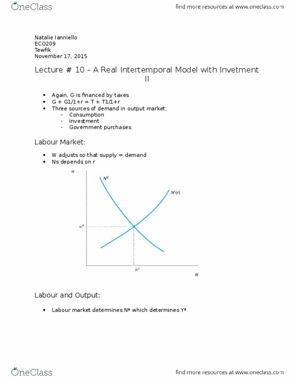
ECO209Y5 Lecture Notes - Lecture 9: Demand Curve, Competitive Equilibrium

Document Summary
Lecture #9 real intertemporal model with investment. They can finance purchases with taxes or with debt. Debt must be paid off in period 2. G + g1/1+r = t + t1/1+r. To find the competitive equilibrium we focus on period 1 because period 2 works like one-period model. W adjusts so that supply = demand. Labour market ns depends on r, nd has nothing to do with r. We want output supplied as a fraction of r r2 > r1, ns shifts up. Therefore, we can graph the output supply curve in terms of r, y(r) Decrease in ns = n* = decrease in y* Increase in wealth = decrease in ns(r) (i. e. labour supply shifts down) Increase in z = increase in y and mpn increases. Therefore, labour demand shifts right = increase in y* Increase in k = y shifts up and mpn increases. Therefore nd shifts right = increase in y*