CAS MA 115 Lecture Notes - Lecture 7: Random Variable, Regional Policy Of The European Union, Normal Distribution

1 May 2018
School
Department
Course
Professor

CHAPTER 7 – THE NORMAL PROBABILITY DISTRIBUTION
Section 7.1 – Properties of the Normal Distribution
Objective 1 – Use the Uniform Probability Distribution
• Uniform Probability Distribution – when a random variable X can be any value within
two equally likely intervals (of equal length)
o ex: what is the probability of a package arriving between 10:00 and 11:00?
o
• Probability Density Function (PDF) – an equation used to compute probabilities of
continuous random variables
o Two Properties:
▪ The total area under the equation graph over all possible values of the
random variable must = 1
▪ The height of the equation graph must be greater than or equal to 0 for all
possible values of the random variable
o The area under the graph of a density function over an interval represents the
probability of observing a value of the random variable in that interval
▪ ex: what is the probability of a package arriving between 10:15 and 10:30?
o It is always true that the probability of a single value will be 0
o This is why there is no difference between x > 4 and x ≥ 4
Objective 2 – Graph a Normal Curve
• When a relative frequency histogram is symmetric and bell-shaped it has a normal curve
find more resources at oneclass.com
find more resources at oneclass.com

• When a continuous/random variable is normally distributed its relative frequency
histogram of the random variable will be bell-shaped and symmetric
o This will make it acceptable to use the empirical rule
Objective 3 – State the Properties of the Normal Curve
• Properties of the Normal Density Curve
o 1. It is symmetric about its mean (μ)
o 2. Because mean = median = mode, the curve has a single peak and the highest
point occurs at x = μ
o 3. It has inflection points at μ − σ and μ + σ
▪ At μ − σ, the graph changes from concave up to concave down
▪ At μ + σ, the graph changes from concave up to concave down
o 4. The area under the curve is 1
o 5. The area under the curve to the right of μ equals the area under the curve to the
left of μ, which equals 0.5
o 6. As x increases (grows larger), the graph approaches, but never reaches, the
horizontal axis
o 7. As x decreases (grows smaller), the graph approaches, but never reaches, the
horizontal axis
o 8. The Empirical Rule:
▪ Approximately 68% of the area under the normal curve is between x = μ −
σ and x = μ + σ
▪ Approximately 95% of the area is between x = μ − 2σ and x = μ + 2σ
▪ Approximately 99.7% of the area is between x = μ − 3σ and x = μ + 3σ.
o 9. When you change μ, the curve will shift right or left along the x-axis
o 10. When you change σ, the curve will stretch or compress along the y-axis
o Larger σ – implies data that is more spread out
o Smaller σ – implies data that is closer together
Objective 4 – Explain the Role of Area and the Normal Density Function
• The area under the normal curve for any interval of values of the random variable X
represents either:
o The proportion of the population with the characteristic described by the interval
of values
o The probability that a randomly selected individual from the population will have
the characteristic described by the interval of values
• ex: the area under the normal curve to the left of x = 2100 pounds is 0.3085. Provide two
interpretations of this result.
o The proportion of giraffes whose weigh is less than 2100 pounds is 0.3085, the
probability that a randomly selected giraffe weighs less than 2100 pounds is
0.3085, about 31 giraffes will weigh less than 2100 pounds.
Section 7.2 – Applications of the Normal Distribution
Objective 1 – Find and Interpret the Area Under a Normal Curve
find more resources at oneclass.com
find more resources at oneclass.com
Document Summary
Section 7. 1 properties of the normal distribution. Objective 3 state the properties of the normal curve: properties of the normal density curve, 1. It is symmetric about its mean ( : 2. Because mean = median = mode, the curve has a single peak and the highest point occurs at x = : 3. The area under the curve is 1: 5. The area under the curve to the right of equals the area under the curve to the left of , which equals 0. 5: 6. As x increases (grows larger), the graph approaches, but never reaches, the horizontal axis: 7. As x decreases (grows smaller), the graph approaches, but never reaches, the horizontal axis: 8. When you change , the curve will shift right or left along the x-axis: 10. When you change , the curve will stretch or compress along the y-axis: larger implies data that is more spread out, smaller implies data that is closer together.