18.03 Lecture Notes - Lecture 10: Ordinary Differential Equation, Partial Differential Equation, Homogeneous Function

1 Introduction to Differential Equations
A differential equation (DE) is an equation relating an unknown function to some of its derivatives.
Many natural laws in engineering, chemistry, biology, physics, economics, etc. can be modeled using DEs.
Objectives
!Identify linear first order differential equations—meaning the we are only dealing with the first derivative
!Use first order linear differential equations to model some system behavior
!Interpret the terms in an ODE as the input signal and system response
!Check reasonableness of models using unit analysis
A Secret Function
!Can you guess the function y(t) that satisfies the DE y' = 3y.
!!y = is a solution to the differential equation because substituting it into the DE gives
!!The general solution to this DE is y =
!Clue: the function satisfies the initial condition y(0) = 5
!!From this we know that y =
!!!This is a particular solution that satisfies the initial condition
Classification of Differential Equations
!An ordinary differential equation (ODE) involves derivations of a function of only one variable
!!Often times the independent variable will be time
!A partial differential equation (PDE) involves partial derivatives of a multivariable function
!Note: the dot notation for derivatives is reserved specifically for time derivatives
!The order of a DE is the highest n such that the nth derivative of the function appears
More Terminology
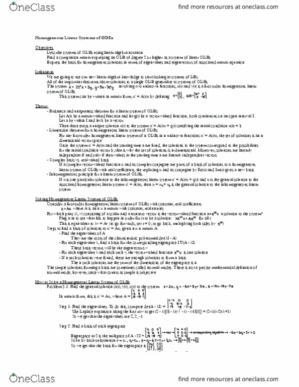
!Homogeneous: A homogeneous linear ODE is a differential equation in which each summand is a function of t time y, y', y"
!!Example:
!!Most general nth order homogeneous linear ODE:
!Inhomogeneous: An inhomogeneous linear ODE is the same exact that it also has one term that is a function of t only; this function is
!usually moved the the right hand side
!!Example:
!!Most general nth order inhomogeneous linear ODE:
!!Imagine feeding different "input signals" q(t) into the right hand side of an inhomogeneous of an inhomogeneous linear
!!ODE to see what "output signals" y(t) the system responds with
!A linear ODE is an ODE that can be rearranged into either of the two types above
!!To simplify slightly, divide the whole equation by the leading coefficient to get rid of it:
!If you already know if an ODE is linear, there is an easy test to decide if it is homogeneous or no. Plug in the function y = 0
!!- If y = 0 is a solution, the ODE is homogeneous
!!- If y = 0 is not a solution, the ODE is inhomogeneous
!For an ODE to be nonlinear, the functions y, y' must enter the equation in a more complicated way: raised to powers, multiplied
!by each other, or with nonlinear functions applied to them
!!Examples:
Introduction to Modeling
!Mathematical modeling is converting a real-world problem into mathematical equations
!- Identify relevant quantities, both known and unknown, and give them symbols and find their units
!- Identify the independent variable(s). The other quantities will be function of them, or constants. Often time is the only IV.
!- Write down equations expressing how the functions change in response to small changes in the independent variable(s).
!- Write down any "laws of nature" relating the variables
!
A Savings Account
!I have a savings account earning interest compounded daily, and I made frequent deposits or withdrawals into the account.
!Find an ODE with initial condition to model the balance.
!Let's assume that interest is paid continuously instead of at the end of each day. Similarly, let's assume that my deposits and withdrawals are frequent
!enough that they can approximated by a continuous money flow at a certain rate, the savings rate.
!Finally, let's assume that the interest rate and savings rate vary continuously with time, but do not depend on the balance.
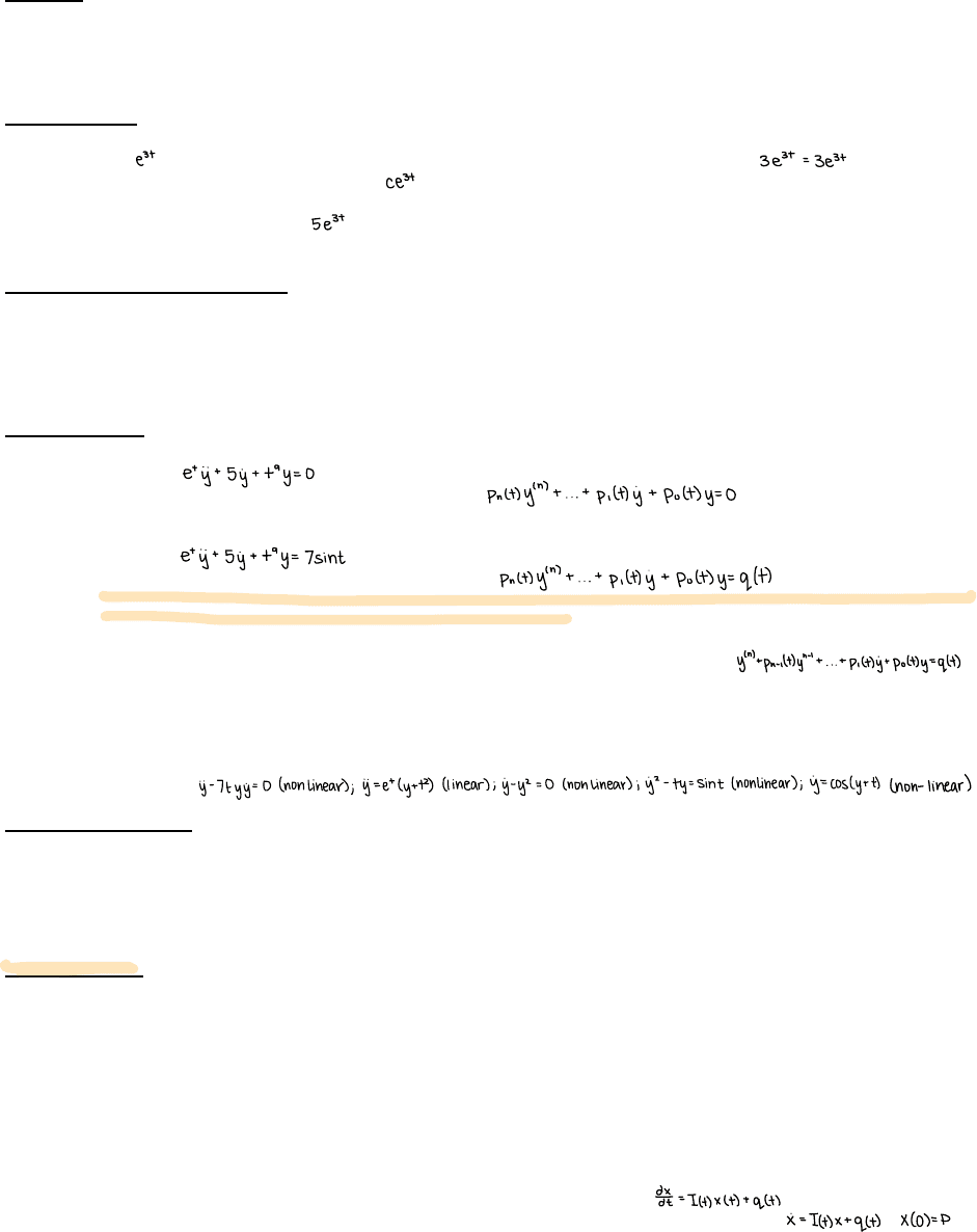
!Variables and functions with units: here t is the independent variable, P is a constant, and x, I, q are functions of t
!!P the principal (dollars), t time (years), x balance (dollars), I interest rate (1/year), q saving rate (dollars/year)
!During a time interval [t, t+Δt] for any positive number Δt:
!!Interest earned per dollar ≈ I(t)Δt, interest eared ≈ I(t)x(t)Δt; amount deposited into the account ≈ q(t)Δt
!!Change in balance ≈ I(t)x(t)Δt + q(t)Δt; change in balance over change in time Δx/Δt ≈ I(t)x(t) +q(t)!
!As Δt —> 0, the approximation becomes exact, yielding the differential equation
!Remember we have the initial condition that x(0) = P, thus we have our ODE with initial condition:

Systems and Signals
!Maybe for financial planning I am interested in testing different saving strategies (different functions q) to see what balances x
!they result in
!In the "system and signals" language of engineering q is the input signal, the bank is the system, and x is the output signal
!The input signal is a function of the independent variable alone, a function that enters into the DE somehow (usually RHS)
!The system processes the input signal by solving the DE with the given initial condition
!The output signal (also called the system response) is the solution to the DE
Cell Division
!Model the number of yeast cells in a batch of dough.
!The first step is to define our variables, the units, and give them names
!!y the number of cells, t time measured in seconds
!We also need to set some initial condition y(0), the number of cells that we begin with at t =0.
!The derivative of y represents the rate at which the number of cells is growing
!We can make this into a true equation by simply inserting a proportionality constant a, such that
!A solution to the above equation is , where C is the number of yeast cells at t = 0
Natural Growth a Decay Equations
!Basic growth equation is , when a is a positive constant.
!Basic decay equation is , when a is a positive constant
Newtonian Mechanics
!Newton's second law is F = ma, which says that force equals mass times acceleration
!!In many cases, we assume mass to be constant
!!We also have to remember that acceleration a, in the case of a 1D system, is the second derivative of the position x
!A mass attached to a spring will feel a force F = -kx, which is a function of the displacement x away from the neutral position
!If the mass is being slowed down by air resistance, we get F = -bx', which is a function of the velocity (x')
!Additionally, the mass experiences a force due to the effects of gravity, F = -mg (assuming positive x is up)
!We can combine these effects if they are all present, getting an equation of the form!
!!This equation is inhomogeneous because x = 0 is not a solution
Solving a First-Order ODE
Objectives
!The solution to a first order linear differential equation given an initial value is a function
!The general solution to any homogeneous first order ODE using separation of variables
!There are infinitely many solution functions to a homogeneous first-order linear differential equation
!!They are all constant multiples of one nonzero solution
!Find solutions to any inhomogeneous first order differential equation by first finding the solution to the associated
!homogeneous function, finding one particular solution, and applying superposition
!Find the particular solution to any inhomogeneous first order ODE using integrating facts and variation of parameters
!
Separation of variables
!Separation of variables is a technique that quickly solves some simple first-order ODEs
!- Check that the DE is a first order ODE. If it is, then proceed with this method of solving
!- Rewrite y' as dy/dt
!- Move terms to the other side of the DE so that the determ with dy.dt is on the left and all other terms are on the right
!- Try to separate the y's and the t's. Specifically, try to multiply/divide and move the dt to the RHS so that it ends up and an
! equality of differentials of the form f(y)∂y = g(t)∂t
!Note: if there are factors with both variables, such as y + t, then it is impossible to separate variables, so use another method
!Warning: dividing the equation by an expression invalidates the calculation if that expression is 0, so at the end, check what
! happens if the expression is 0; this may add to the list of solutions
!- Integrate both sides to get an equation of the form F(y) = G(t) + C
!- If possible (and if desired), solve for y in terms of t
!- Check for extra solutions by checking what happens if the expression is 0
!- Check your work by verifying that the general solution actually satisfies the original ODE
!Example:
!!Check what happens when y = 0:
!!General solution:
!!Check: plug in
Standard Form
!Homogeneous: y' + p(t)y = 0!Inhomogeneous: y' + p(t)y = q(t)

!Homogeneous first-order linear ODE can always be solved by separation of variables
!!y' + p(t)y = 0 —> ∂y/∂t = -p(t)y —> ∂y/y = -p(t)∂t —> ln|y| = -P(t) + C —> |y| = ±e —> y = ce
!Suppose that x is a solution to the differential equation x' + p(t)x = 0 and that x (a) < 0 at some t = a. This tells us that the
! function x has a negative value at all t. The solution had the form x = ce for some constant c and some antiderivative
! P(t) of p(t). The value e is positive, but x (a) < 0, so c must be negative, and then x = ce < 0 for all t
Inhomogeneous Equations: Variation of Parameters
!Variation of parameters is a method for solving inhomogeneous linear ODEs y' + p(t)y = q(t):
!- Find a nonzero solution, say y , of the associated homogeneous ODE y' + p(t)y = 0
!- For a undetermined function u(t), substitute into the inhomogeneous equation (y' + p(t)y = q(t)) to find out which
! choices of u(t) make this y a solution to the inhomogeneous equation
!- Once the general u(t) is found, multiply it by the homogeneous solution y (t) to find y = u(t)y (t), the general solution
!The idea is that the functions of the for cy are solutions to the homogeneous equation; maybe we can get solutions to the
! inhomogeneous equation by allowing the parameter c to vary, i.e. we replace it by a nonconstant function u(t)
!Example: Solve on the interval (0,∞)
!- Solve the associated homogeneous equation:
!- Substitute into the inhomogeneous equation:
!- The general solution to the inhomogeneous equation is
Inhomogeneous Equations: Integrating factor
!Another approach to solving the first order, linear, inhomogeneous ODE y' + p(t)y = q(t) is the use an integrating factor
!- Find an antiderivative P(t) of p(t)
!- Multiply both side of the ODE by the integrating factor in order to make the left side the derivative of something
!
! Here represents all possible antiderivative of , so there are infinitely many solutions
! If you fix one antiderivative, say R(t), then all others are R(t) + c for a constant c, so the general solution is
Superposition
!A linear combination of a list of functions is any function that can built from them by scalar multiplication and addition
!Superposition principle:
!- Multiplying a solution!!!! by a number a gives a solution of
!- Adding a solution of !!!! to a solution of !! !!!!!!!!!!!!!!!!!!!!!!!!!!!!!!!!! gives a solution of
Consequence of Superposition for a Homogeneous Linear ODE
!Apply superposition with right hand side equal to zero
!Conclusion: the set S of solutions to a homogeneous linear ODE has the following properties
! - The zero function 0 is in S
! - Multiplying any one function in S by a scalar gives another function in S
! - Adding any two functions in S gives another function in S
!A set of functions with these properties is called a vector space of functions, since these properties say that you can scalar-multipy
!and add such function, as you can with vectors.
!For any homogeneous linear ODE, the set of all solutions is a vector space
Consequences of Superposition for an Inhomogeneous Linear ODE
!To understand the general solution y to an inhomogeneous linear ODE, to the following:
!- List all solutions to the associated homogeneous equation (y )
!- Find any one particular solution (y ) to the inhomogeneous ODE
!- Add y to all the solutions of the homogeneous ODE to get all the solutions to the inhomogeneous ODE
!The superposition principle does not hold for nonlinear differential equations
!Suppose that we have two equations x (t) and x (t) that satisfy the homogeneous nonlinear DE
!What input signal q(t) is needed for the function y = x (t) + x (t) to be a solution to the DE?
!!Plug x + x into our differential equation
Newton's Law of Cooling
!Model the temperature of soup in a thermos as a function of time, assuming the insulating ability of the thermos does not
!change with time and the rate of cooling depends only on the difference between the soup temperature and the external temp
!Variables and functions with units: t time (minutes), x external temperature (°C), y soup temperature (°C)
!Equation y' = ƒ(y-x) assuming that ƒ(z) = -kz + l, so we get that y' = -k(y - x) + l
!Common sense that if y = x, then y' = 0. Thus l should be zero
!If y > x, then y is decreasing. This is why we wrote -k instead of just k
!And with all of this taken into consideration, the equation becomes y' = -k(y - x)