STATS 10 Lecture Notes - Lecture 4: Grammatical Number, Standard Deviation, Unimodality


Chapter 3: Numerical Summaries of Center and Variation
Numeric summaries (sample statistics) summarize the data in our sample
● Esp useful when comparing between samples
● E.g. GPA is a singular number tha tsummarizes academic performance, GDP is a measure of country’s economic
health
● For any dataset, often 2 numeric sum values are enough: CENTER (typical values) and SPREAD (variability)
Center of a distribution is where typical/common (“average”) values tend to be
● Two different ways to think about center:
○ Balancing point (center of mass)
○ Halfway point
● Our idea of what typical/avg means depends on how data is distributed; depends on shape of distribution
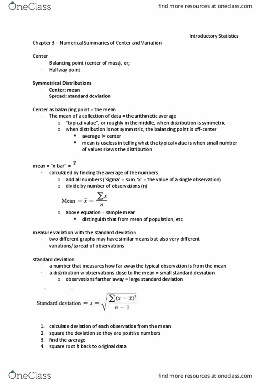
Mean: arithmetic average of data values, most commonly used measure of center
● Aka balancing point of distribution (think of a fulcrum/seesaw thing)
○ When distribution of data is roughly symmetric, mean closely matches our concept of
“typical value”
■ WARNING: May not match typical value when distribution is highly skewed;
plot data first to see if you should use the mean as a measure of center
● X-bar (x
̅) =mean aka sample mean; n=sample size (number of observations)
Spread of a distribution is how much variability there is in values, i.e. how spread out the data is
● How far away from the center is still “typical”? Look at both center and spread!
● Standard deviation is a number that measures how far away the typical observation is from the mean
○ Relatively many observations at large distance from mean (wide spread) → larger standard dev.
○ Relatively many observations at small
distance from mean (clustered near
mean) → smaller stddev
○ RULE OF THUMB (for symmetric and
unimodal distr.): the majority (~⅔) of
observations are less than one standard dev from the mean
○ Denotated by s
● variance=standard dev squared: s2
○ Lots of theoretically useful properties but in practice, standard dev (s) is
preferred over variance (s^2)
○ Standard dev=same units of measurement as mean and data values
○ variance=squared units, harder to interpret
The Empirical Rule: a rule of thumb that helps us understand how standard dev. Measures variability
● If distribution is symmetric/unimodal, then
○ Approx 68% of observations (~⅔) will be within 1 standard dev of the mean
○ Approx 95% of the observations will be within 2 standard devs of the mean
○ Nearly all observations will be within 3 standard devs of the mean
● The more symmetric/unimodal the distribution, the better the predictions from this rule tend to be
○ Does NOT apply when distribution is highly skewed/multimodal
Unusual values
● Statisticians often consider data values that occur 5% of the time or less (ie values outside 2 standard devs from
the mean) are “unusual” or “rare”
○ What is considered unusual will depend on context
Standard Units and z-scores
● Standard unit measures how many standard deviations away an observation is from the mean
○ Z-score: measurement converted to standard units; measures distance from mean in units of standard
dev
■ Z-score of 1.0: one standard dev from mean
■ Z-score of -2.2: 2.2 standard devs below mean
find more resources at oneclass.com
find more resources at oneclass.com
Document Summary
Chapter 3: numerical summaries of center and variation. Numeric summaries (sample statistics) summarize the data in our sample. Gpa is a singular number tha tsummarizes academic performance, gdp is a measure of country"s economic health. For any dataset, often 2 numeric sum values are enough: center (typical values) and spread (variability) Center of a distribution is where typical/common ( average ) values tend to be. Two different ways to think about center: Our idea of what typical/avg means depends on how data is distributed; depends on shape of distribution. Mean: arithmetic average of data values, most commonly used measure of center. Aka balancing point of distribution (think of a fulcrum/seesaw thing) When distribution of data is roughly symmetric, mean closely matches our concept of. Warning: may not match typical value when distribution is highly skewed; plot data first to see if you should use the mean as a measure of center.