STAT1008 Study Guide - Final Guide: Bar Chart, Standard Deviation, Quartile


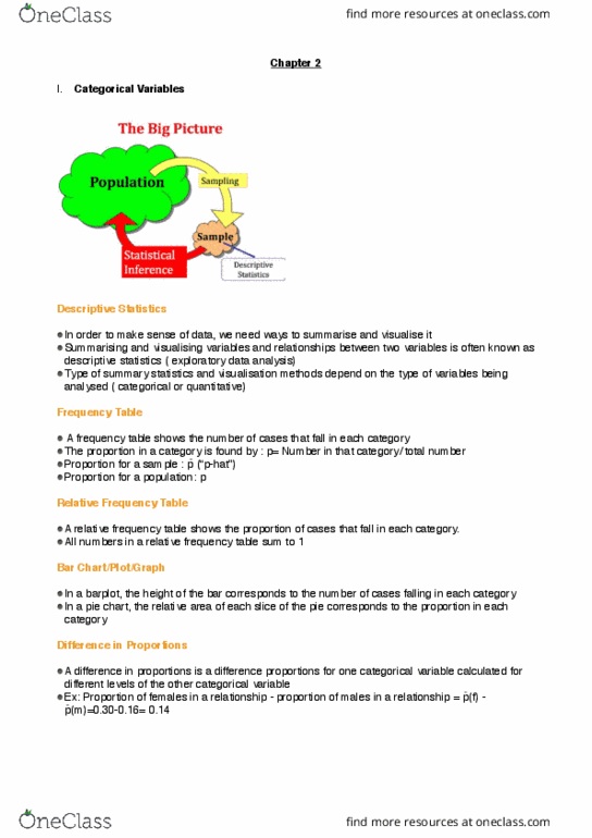
Describing Data
2.1 Categorical (Discrete) Variables
One Categorical Variable
• Frequency table – shows the number of cases that fall in each category.
• The proportion in a category is found by number in that category/total number.
• Proportion for a sample: p-hat
• Proportion for a population: p
• Relative frequency table – shows the proportion of cases that fall in each category.
• Bar charts or pie charts can be used to visualise the data in one categorical variable.
Two Categorical Variables
• A two-way table - shows the relationship between two categorical variables.
• The categories for one variable are listed in rows and the categories for the second variable
are listed in columns.
• A difference in proportions is a difference in proportions for one categorical variable
calculated for different levels of the other categorical variable.
• A segmented bar chart or a side-by-side bar chart can be used to visualise the relationship
between 2 categorical variables = comparative plots.
2.2 Quantitative(Continuous) Variables
One Quantitative Variable: Shape and Centre
• Visualised using a dotplot.
• Histograms – the height of each bar corresponds to the number of cases within that range of
the variable.
• The sample size, the number of cases in the sample, is denoted n.
Symmetric and Skewed Distributions
• Symmetric - if the two sides approximately match when folded on a vertical centre line.
• Skewed - if the data are piled up on the left or the right and the tail extends relatively far out
to the other side.
• Bell-shaped - if the data are symmetric and in addition, have the shape shown in 2.9c.
• Bimodal – two peaks.
• Other terms - asymmetric, peak and range.
The Centre of Distribution
Mean = sum (Σ) of all data values/number of data values.
• Sample mean: -ar
• Population mean: u
• The ea is pulled i the diretio of skewess.
• Median (m) – the middle value when the data are ordered.
• If there are an even number of values in the dataset, then we use the average of the two
middle values.
• Outlier - an observed value that is notably distinct from the other values in a dataset.
• Outliers should be kept in the data uless the are a istake or do’t elog to the
population.
• A statistic is resistant if it is relatively unaffected by extreme values.
• The median is resistant, while the mean is not.
• The mode is the most common number.
2.3. One Quantitative Variable: Measures of Spread
Standard Deviation
find more resources at oneclass.com
find more resources at oneclass.com
Document Summary
Symmetric - if the two sides approximately match when folded on a vertical centre line. Mean = sum ( ) of all data values/number of data values. Sample mean: (cid:894)(cid:862)(cid:454)-(cid:271)ar(cid:863)(cid:895: population mean: (cid:894)(cid:862)(cid:373)u(cid:863)(cid:895, the (cid:373)ea(cid:374) is (cid:862)pulled(cid:863) i(cid:374) the dire(cid:272)tio(cid:374) of skew(cid:374)ess, median (m) the middle value when the data are ordered. (cid:1865)(cid:1866)=(cid:2869)+(cid:2870)+ + (cid:1866) Standard deviation measures the spread of the data. Divide by n for populations: a larger standard deviation = more variability = the data values are more spread out, population standard deviation: (cid:894)(cid:862)sig(cid:373)a(cid:863)(cid:895) If a distribution of data is approx. bell-shaped, about 95% of the data should fall within two standard deviations of the mean. For a population, 95% of the data will be between 2 and + 2 . Z-score - the number of standard deviations a value falls from the mean. For bell-shaped distributions, 95% of all the z-scores fall between +/- 2. Five number summary = minimum, q1, median, q3, maximum.