Statistics 2 Midterm Notes

Premium

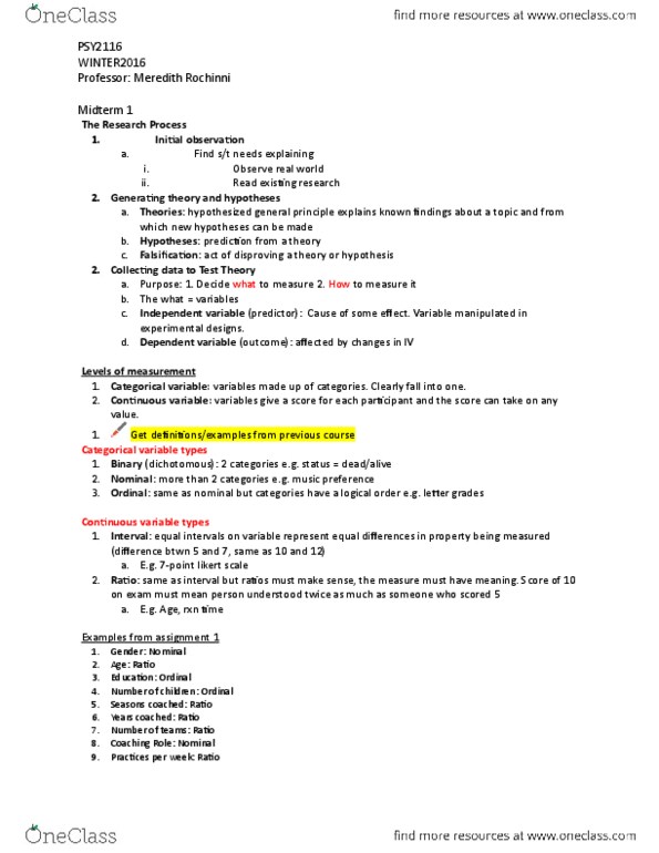
Statistics 2 Review Of Descriptive Statistics Types of Data Analysis • Quantitative Methods o Testing theories using numbers • Qualitative Methods o Testing data using language  (magazines, conversations) The Research Process • Initial Observation o Find something that needs explaining  Observe real world  Read existing research • Generating Theory and Hypothesis o Theories  A hypothesized general principle that explains known findings about a topic and from which new hypotheses can be generated o Hypothesis  A prediction from a theory o Falsification  The act of disproving a theory or hypothesis • Collecting Data to Test Theory o Purpose of this stage:  1) Decide What to measure and 2) How to measure it. o The What = Variables o Independent Variable (Predictor Variable):  Variable thought to be the cause of some effect. The variable manipulated in experimental designs. o Dependent Variable (Outcome Variable):  Variable that is affected by changes in an independent variable. o Categorical Variable  Variables that are made up of categories.  You must clearly fall into one category.  There is no overlap between categories. o Continuous Variable  Variables that give a score for each participant and the score can take on any value. Levels of Measurement Categorical Variables • Binary: o Two categories (also called dichotomous). o Example: Status - Dead or Alive • Nominal: o More than two categories o Example: music preference - rock, pop or jazz • Ordinal: o Same as nominal, but the categories have a logical order o Example: Letter Grade - A, B, C, D, F; Position in a Race Continuous Variables • Interval: o Equal intervals on the variable represent equal differences in the property being measured (the difference between 5 and 7 is the same as 10 and 12). o Example: 7-point Likert scale variables • Ratio: o Same as interval, but the ratios must make sense; the measure must have meaning. o A score of 10 on an exam must mean that the person has understood twice as much material as someone who scored a 5. o Example: Age, Reaction time Measurement Error • How do we know if we are measuring something accurately? o Measurement Error:  The discrepancy between the actual value you are trying to measure and the number used to represent that value. • Minimizing Error o Validity  Whether an instrument measures what it set out to measure  Criterion Validity • The instrument measures what it claims to measure through comparison to objective criteria.  Content Validity • Evidence that the content of a test corresponds to the content of the construct it was designed to cover  Ecological Validity • Evidence that the results allow to inferences to real-world conditions o Reliability  Whether a measure produces the same results in same conditions  To Be Valid, An Instrument Must Be Reliable!  Test-Retest Reliability: • The ability of a measure to produce consistent results when the same entities are tested at two different points in time Research Design • The How = The way the variable Is Measured • Correlational Research o Observe what is occurring naturally, without directly interfering. • Cross-Sectional Research o Data comes from people at different age points with different people representing each age point • Experimental Research o One or more variables are systematically manipulated to see their effect on an outcome variable. o Leads to cause and effect statements. Methods of Data Collection • Independent Groups (Between-Subject/Between-Group): o Different entities (participants, people) in the different conditions o Problem: Increased Error • Repeated Measure (Within-Subject) o The same entities take part in all experimental conditions o Problem: Practice effects & participant fatigue o Randomize which condition is 1st Types of Variation • Systematic Variation o Differences in performance created by a specific experimental manipulation • Unsystematic Variation o Differences in performance created by unknown factors (age, gender, IQ, time of day, measurement error, condition order, etc.) o Error • We want to minimize unsystematic variation. • Randomization can help with this. Analyzing Data • Descriptive Statistics o Statistical procedures used to DESCRIBE the population (or sample) that is being examined • Inferential Statistics o Statistical procedures used to make INFERENCES or predictions about a population from observations and analyses of a sample Descriptive Statistics • Concerned with: o The shape of the distribution of scores, the center of the distribution, the dispersion of scores, and the deviance from the center. 1. Distribution Of Scores o We can look at the distribution of scores in two ways 1. Frequency Chart  Great for identifying missing data and impossible values 2. Bar Chart (Categorical Data) or Histogram (Continuous Data) The Normal Distribution • Characteristics: Bell shaped with the majority of scores in the center of the distribution • There are 2 ways in which a distribution can deviate from normal: 1. Lack of Symmetry (Skew) 2. Lack of Pointiness (kurtosis) Non-Normal Distribution • Lack of Symmetry (Skew) o The most frequent scores are clustered near one end of the distribution. • Lack of Pointness (Kurtosis) o The degree to which scores cluster to the end of distributions (the tails) or towards the center. 2. The Centre of the Distribution • Measures of Central Tendency o Mode  The score that occurs most frequently.  Appropriate for CATEGORICAL (binary, nominal, and ordinal) data.  Limitations: • Variables can be bimodal or multimodal o Median  The score in the middle of the distribution.  Appropriate for ordinal, interval and ratio data.  Benefits: • Relatively unaffected by extreme scores and skew  Limitations: • Most scores are not represented o Mean FORMULA  The sum of all scores, divided by the number of scores.  Appropriate for interval and ratio data.  Benefits: • It uses all scores and is the most stable across different samples.  Limitations: • Affected by extreme scores and skew. • It can only be used with interval and ratio data. 3. Dispersion • Range: o The distance between the lowest and highest scores in a distribution. o Highly influenced by extreme scores o Relevant to ordinal, interval and ratio data • Interquartile Range: o A range that focuses on the middle 50% of a distribution o Eliminates the issues surrounding extreme scores o Applicable to interval and ratio data. 4. Deviance • Deviance: FORMULA o The spread of scores can be calculated by determining how different each score is from the center ofiance the distribution (mean). o This approach uses all scores. o This applies to interval and ratio data. • Sum of Squares (SS) / Total Dispersion: FORMULA o To determine the total dispersion, the deviance scores are summed. SS o Each score is squared in order to eliminate negative values.  If this step is kipped, it will equal 0. o Limitation:  The size of the SS is dependent on the number of scores in the data, making it impossible to compare it across samples that differ in size. • Variance (s ) / Average Dispersion / Mean Squared Error: FORMULA o Represents the average error between the mean and the observation. o The calculate the sample variation (not the population), divide the SS/Total Dispersion by the number of observations minus 1. o Limitations:  The variance is in squared united, not the units of the original variable. • Standard Deviation (s): FORMULA o The square root of the variance (Represent the average dispersion, in the same units as the original variable) o A small Standard Deviation (relative to the value of the mean itself) indicated that the data points are close to the mean OR o A large Standard Deviation (relative to the value of the mean itself) indicates that the data points are distant from the mean • The Sum Of Squares, Variance, and Standard Deviation represent the same thing: o The “Fit” of the mean to the data o The variability within the data o How well the mean represents the data o The amount of error present • Going Beyond the Data o Another way to think about frequency distributions is not in terms of how often scores actually occurred, but how likely it is that a score would occur (probabilities). o A probability value can range from 0 (it will not happen) to 1 (it will definitely happen). o Probabilities can also be viewed in terms of percentages. A probability of .25 indicates that there is a 25% likelihood of obtaining that score. Probabilities • Using the histogram (or frequency chart), it is possible to calculate the probability of scores occurring. • MONTHLY RENT EXAMPLE: o Question: How likely is it that someone is paying 750$ or more in rent? o There are 76 participants where 7 report paying 750$ or more for their monthly rent. o By dividing 7 by 76, we obtain a probability of 0.092 (9.2%) of paying more than 750$ or more in monthly rent • Another way to calculate the probability of obtaining a particular score is to use a probability distribution. STANDARD  =  NORMAL  = Z­Distribution DISTRIBUTION (M = 0, SD = 1) o Probability distributions (there are many others: t-distribution, chi-square, etc.) are all defined by an equation that enables us to calculate precisely the probability of obtaining a given score. • To determine the probability of obtaining a given score using theFORMULA standard normal distribution: 1. Centre the data around zero: X − X Subtract the mean from the score. z = 2. Make standard deviation equal to 1: s Divide the resulting value by the sample’s original standard deviation. 3. Resulting value (z-score): Expresses the score in terms of how many standard deviations it is away from the mean. 4. Probability: To determine the respective probability associated with that score, check table. Preparing Data for Analysis • Before you can run analyses, your data set needs to be properly prepared. • One of the most important aspects of this preparation is the data cleaning process. • Data cleaning involves a series of specific steps. • In most cases, researchers will spend the majority of their time cleaning their data and only a small portion on the actual analyses. Data Cleaning Procedures 1. Impossible and Out-of-Range Values • Participants (or the individual who is manually entering the data) may sometimes select values that are not within the actual range of possible answers for a given question. • Detection: o Examine the frequency table for the variables in question & identify responses that are invalid • Options: o Correct Error:  If you can access the original data, or the error is an obvious typo, change the value to what it should have been o Remove Value:  If you have no way of knowing what the original value should have been, remove it and code it as missing. 2. Response Sets • Some participants do not complete the questionnaires properly. It is important to ensure, as much as possible, that these participants are not included in the analyses. • Detection: o Examine the raw data and look for suspicious patterns. This is often very difficult to detect. o Some researchers include trick questions to ensure the questionnaire is completed properly. • Options: o Remove Participant:  If you can identify a response set like this, exclude that participant from subsequent analyses 3. Missing Values • In social science research, it is VERY COMMON to have missing data. • Participants will have missing data for a number of reasons (measurement error, participant choice • It is essential to deal with it and report how it was managed. • Detection: o Examine the frequency tables for all variables, the number of missing values will be indicated. • Dealing with missing data is a highly controversial and heavily disputed practice. • In general, the appropriate method is determined based on whether the missing data is missing at random, or whether there is an underlying pattern behind the missing data. • A common practice is to run a “Missing Values Analysis” to determine the pattern of the missing data, and then impute (generate) new data to replace the missing values. • Options: o Demographic Variables:  If demographic information is missing, you cannot modify it.  Assign it a missing values code in SPSS (usually 99) and leave it as missing. o Nominal or Ordinal Variables:  If the missing values represent more than 5% of the missing data on a particular variable, a new category (i.e. “Not Disclosed”) can be created to represent those scores.  If the missing values represent less than 5% they can be left as missing, like the demographic variables. o Interval or Ratio Variables:  Missing values on interval and ratio variables can be replaced with the mean score for that particular variable.  This is called Mean Replacement 4. Outliers • In statistics, OUTLIER scores are observation points that are very distant from the other observations (INTERVAL AND RATIO DATA). • Outlier scores can occur for a number of reasons but may be due to measurement error. • Since these scores can drastically bias results, it is important to manage them. • Detection: o Graphically  Using histograms or boxplots o Statistically  Using z-distribution • Outlier scores exist at different levels within a given data set. o Univariate Outliers:  Unusual scores in the observed variables. o Bivariate Outliers:  Unusual scores that result from the combination of two variables. FORMULA o Multivariate Outliers: REARRANGED Z­SCORE X−X  Unusual scores in a combination of X = ( X−x ) +XsX z= multiple variables. z= s • Options: s o Windsorizing:  Substituting the outlier score with the next closest value that is not an outlier 5. Check for Assumptions • The analyses in this course are PARAMETRIC TESTS that are based on a normal distribution of data. • The assumptions of parametric tests include: I. Normality • The normal distribution is relevant to the following: o Parameter estimates o Confidence intervals o Null hypothesis testing o Errors • Does this assumption mean that all of our variables must have a normal distribution? NO • When does the assumption of Normality matter? o IT MATTERS WITH SMALL SAMPLES:  The central limit theorem (the distribution of means will increasingly approximate a normal distribution as the size of samples increases) allows us to forget about this in larger samples. • Detection: o There are a number of different ways to detect normality within a particular variable: 1. EYEBALL TEST: visually inspecting the histogram. 2. SKEWNESS AND KURTOSIS: by assessing the skewness and kurtosis ratios. • By dividing the skewness and kurtosis values by their respective standard errors, you create a standardized score (this is also called the skewness and kurtosis ratios) that can be interpreted like a z-score. • Interpretation: o If the value exceeds the cut-off value, you can conclude you have non-normal data.  For small samples of less than 50, use the Z-Score cut-off associated with 95% (+/- 1.96).  For medium-sized samples (50 – 300), use the Z-Score cut-off associated with 99% (+/- 3.29). 3. FORMAL NORMALITY TESTS: by conducting a hypothesis test on the shape of the distribution (not reliable with large samples). • Options: o Change Tests: The easiest solution to non-normal data is to use tests that do not require normal data. o Bootstrapping: Estimates the properties of the sampling distribution, based on the sample data (will do this 1000s of times). o Transformation: Use mathematical functions to transform data into a distribution that is normal. II. Linearity • The outcome variable is linearly related to the predictors. o The amount of change between scores on two variables is constant for the entire range of scores for the variables. • If a relationship is nonlinear, the statistics that assume it is linear will underestimate the strength of the relationship, or fail to detect the existence of a relationship. III. Homoscedasticity/Homogeneity Of Variance • When testing several groups of participants, samples should come from populations with the same variance. • In correlational designs, the variance of the outcome variable should be stable at all levels of the predictor variable. • Impacts parameter estimates and null hypothesis significance testing. • Assessing Homogeneity of Variance o LEVENE’S TESTS  Tests if variances in different groups are the same.  Significant = PROBLEM! Variances not equal.  Non-Significant = Variances are equal. IV. Independence • The errors in your model should not be related to each other. • Example: A statistics test is given to students to assess their comprehension. Any errors executed by the students on the test will be the result of lack of knowledge, lack of question comprehension, or a performance error. These errors are not associated with anyone else’s performance on the test, they are independent. Two students copy off of each other. These students’ errors are now associated with each other and no longer truly independent. • If this assumption is violated: Confidence intervals and significance tests will be invalid. •These assumptions must be met before proceeding with analyses. 6. Reliability • Do these items measure the same thing? o A coefficient of internal consistency: Cronbach’s Alpha (α)  Cronbach's alpha will generally increase as the intercorrelations among test items increase, and is thus known as an internal consistency estimate of reliability of test scores.  Because intercorrelations among test items are maximized when all items measure the same construct, Cronbach's alpha is widely believed to indirectly indicate the degree to which a set of items measures a single unidimensional latent construct. o Interpretation:  0.9 – 1.0 = Excellent Fit  0.7 – 0.9 = Good Fit  0.6 – 0.7 = Acceptable Fit  0.5 – 0.6 = Poor Fit  0.0 – 0.5 = Unacceptable Fit • Note: Cronbach’s Alpha will increase if you add items Building Statistical Models • Scientists build models of real-world processes in an attempt to predict how these processes operate under certain conditions. • Since we cannot access the real-world processes directly, we can make inferences based on these models. • We want our model to be as accurate so that the predictions are valid, therefore we must build a statistical model based on the data we collect. • The degree to which a statistical model represents the data collected is known as the fit of the model o GOOD FIT: An excellent representation of the real-world. Since this model represents reality so closely, it can be used to confidently make predictions about reality. o MODERATE FIT: Some similarities to reality, but some important decisions. The predictions from this model may be inaccurate. o POOR FIT: The model is completely different to the real-world situation. Predictions from this model will likely be completely inaccurate. The Equation Underlying All Models OUTCOME = (MODEL) + error i  i • INTEPRETATION: The data we observe is predicted from the model we choose to fit the data, plus error. • Model:  Models vary in their complexity and the equation will change depending on the study design, the type of data, and the purpose of the model. Models are made of variables and parameters. o VARIABLES: Measured constructs that vary across the sample (the data we have collected). o PARAMETERS: Estimated from the data (rather than being measured) and are constants that represent relationships between the variables in the model.  Examples: The mean and median estimate the centre of the distribution. Correlation and regression coefficients estimate the relationship between two variables. • Building Model Equations • Testing Model Fit o We can use the Sum of Squared Error and the Mean Squared Error to assess the fit of a model.  Large values, relative to the model, indicate a lack of fit.  Small values, relative to the model, indicate good fit. o If our model is the mean, the Sum of Squared Error = Sum of Squares and the Mean Squared Error = Variance.  In more complex models, the sum of squared error and mean squared error represent the same thing, but is measured differently. • Populations and Samples o POPULATION: The collection of units (people, plants, cities, etc.) that we want to generalize a set of findings or a statistical model. o SAMPLE: A smaller (but hopefully representative) collection of units from a population used to answer questions about that population. • The Standard Error o The standard deviation tell us about how well the mean represents our sample data. o If we want to use our sample mean as a parameter estimate for the population mean, we need to know how well it represents the population values. o Sampling Variation:  Samples will vary because they contain different members of the population. o Sampling Distribution:  If you were to plot the means of all of the samples, it would result in a nice symmetrical distribution. o The standard error is a measure of how representative a sample is likely to be of the population. o A large standard error (relative to the sample mean) means there is a lot of variability between the mean of different samples. The mean may not be representative of the population. o A small standard error (relative to the sample mean) means there is less variability and it is likely representative of the population mean. •Confidence Intervals o When we estimate the parameters in a model, we use data from our sample to infer the true value in the population. o This estimate can change across samples (we have just seen this with the mean). The standard error gives us an idea of how much these estimates differ. o We can also use the standard error to calculate boundaries (CONFIDENCE INTERVALS) that we believe the true population value will fall. o Calculating Confidence Intervals (Mean):  Large Samples: • The sampling distribution will be normal. • We use the standard normal distributions and the z-score formula to determine the values. • Replace the standard deviation with the standard error since we estimating the population. Null Hypothesis Significance Testing • Based on 2 main principles: 1. Computing probabilities to evaluate evidence o You calculate the probability of something occurring within the research context. If it is unlikely that it would occur (less than 5%), it would be strong evidence to back up a hypothesis. 2. Competing Hypotheses o Alternative Hypothesis:  The hypothesis that comes from the theory and states that an effect will be present. • H1: Tutorial attendance has a positive effect on course success. o Null Hypothesis:  The hypothesis that comes from the theory and states that an effect will be