STAT 1450 Study Guide - Final Guide: Central Limit Theorem, Point Estimation, Confidence Interval

17 Sep 2020
School
Department
Course
Professor
Chapter 20, page 1
STAT 1450 COURSE NOTES – CHAPTER 20
INFERENCE ABOUT ONE POPULATION MEAN
Connecting Chapter 20 to our Current Knowledge of Statistics
We know the basics of confidence interval estimation (Chapter 16) and tests of significance
(Chapter 17). Nuances that we should be aware of were also presented (Chapter 18).
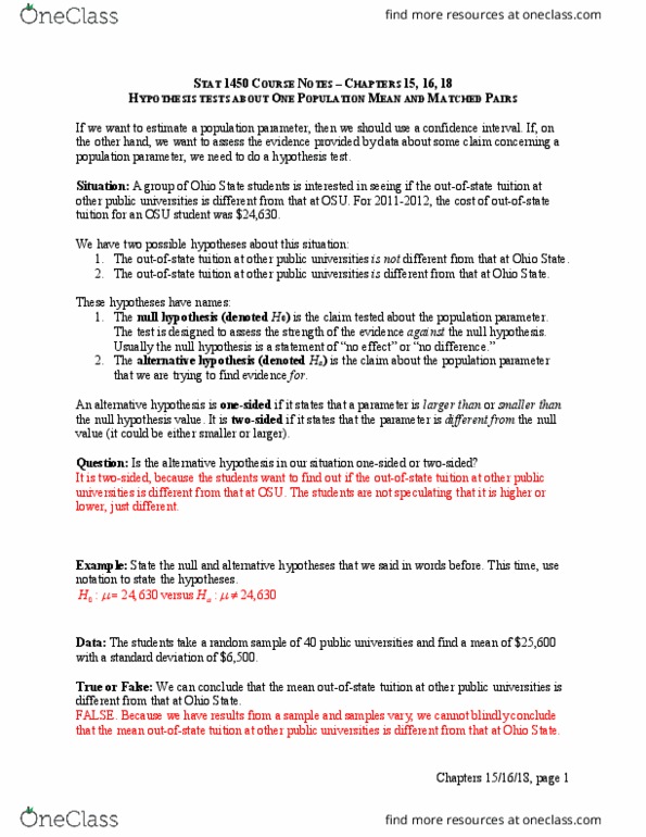
Parameters and their Point Estimates
Measure
Sample Statistic
and Point Estimate
Population
Parameter
̅
P
s
σ
𝑝̂
𝑝
In the coming chapters, we will either find confidence intervals for the population parameters, or,
conduct tests of significance regarding their hypothesized values.
In either case, the point estimates will help us in our endeavors.
It is unlikely that the population standard deviation σ will be known
and the population mean μ will not be known.
Chapter 16 taught us that ̅ is the best point estimate of PSimilarly, s can estimate σ.
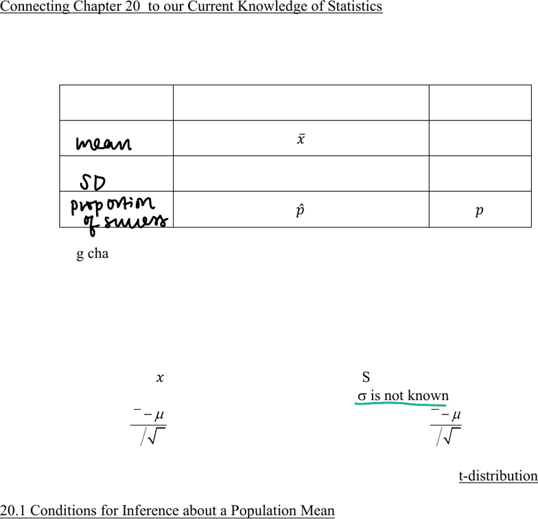
In Chapter 15 when V was known we used: Now when V is not known we can use s instead:
x
zn
P
V
x
tsn
P
This equation follows a This new equation is not quite Normal.
Standard Normal Z-distribution This statistic follows a t-distribution.
20.1 Conditions for Inference about a Population Mean
The conditions for inference about a mean are listed on page 456 of the text.
x Random sample: Do we have a random sample?
If not, is the sample representative of the population?
If not a representative sample, was it a randomized experiment?
x Large enough population : sample ratio:
Is the population of interest 20 times n?
x The population is from a Normal Distribution.
If the population is not from a Normal Distribution, then the
sample size must be large enough with a shape similar to the
Normal Distribution; then we apply the Central Limit Theorem.
mean
SD
proportion
of
success
Chapter 20, page 2
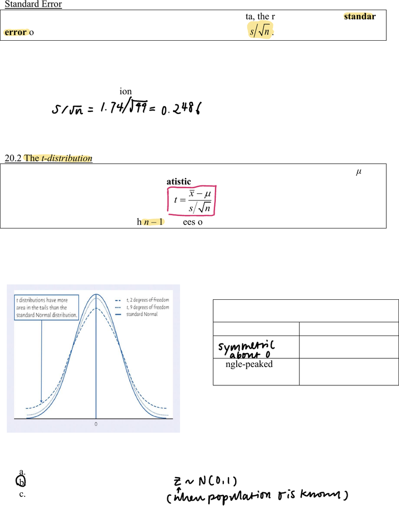
Standard Error
When the standard deviation of a statistic is estimated from data, the result is called the standard
error of the statistic. The standard error of the sample mean is
sn
.
Now the sample standard deviation will replace V in many of our recent formulas; resulting in a
new distribution.
Example: A random sample of 49 students reported receiving an average of 7.2 hours of sleep
nightly with a standard deviation of 1.74. What is the standard error of the mean?
20.2 The t-distribution
Draw an SRS of size n from a large population that has the Normal distribution with mean μ and
standard deviation σ. The one-sample t statistic
x
tsn
P
has the t distribution with n 1 degrees of freedom.
With the sample standard deviation replacing V; we can use the one-sample t statistic for
confidence intervals and tests of significance.
As mentioned earlier, the t-distribution is not quite Normal.
Here is a plot of two t distributions (dashed) and the standard Normal distribution (solid):
Poll: The t2 curve has thicker dashes. The t9 curve has smaller dashes. Z is the solid curve.
What would you anticipate happening to tdf as the degrees of freedom (df) increase?
a. tdf will not be affected
b. tdf will approach Z
c. tdf will become further from Z.
T-Distribution as Compared
with the Z-Distribution
Similarities
Differences
T has thicker tails
Single-peaked &
Bell-shaped
Varies based upon
degrees of freedom
Sir I74474 02486
a
symmetric
about0
DZnNOil
inherr
population oisknown
Chapter 20, page 3
...
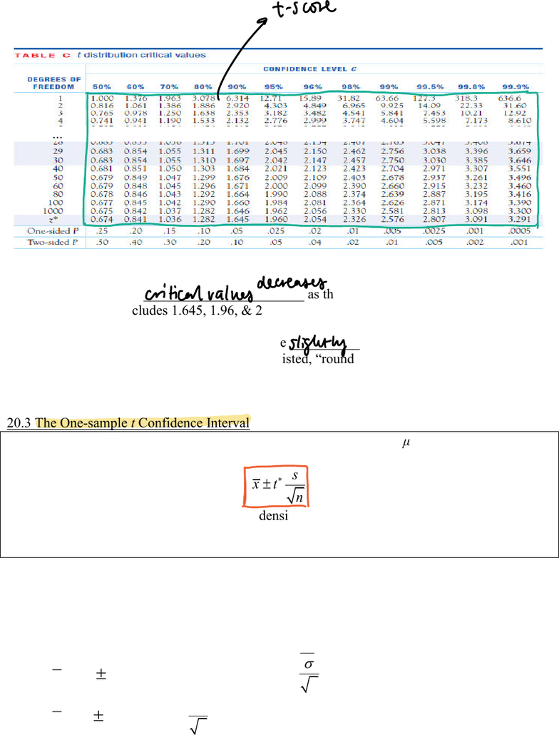
Notes about Table C
1. The t-distribution _______________________ as the degrees of freedom (df) increase.
2. The final row includes 1.645, 1.96, & 2.576. These are common confidence levels & z*.
3. Confidence intervals based upon t will be __________ wider than those based upon z.
4. Be conservative. When the exact df is not listed, round down and use the closest df that
does not exceed the df that is desired.
20.3 The One-sample t Confidence Interval
Draw an SRS of size n from a large population having unknown mean μ.
A level C confidence interval for μ is
s
xt n
r
where
t
is the critical value for the t(n 1) density curve with area C between
t
and
t
.
This interval is exact when the population distribution is Normal and is approximately correct for
large n in other cases.
The one-sample t confidence interval is used to estimate means.
Its form is similar to previous forms of confidence intervals.
____ ___ __________________________ ____________________________
x
r
(1.96, or, another z-score)
n
V
General Form (when V is known)
x
r
s
tn
Now (V is unknown).
ftscore
11
critical
values
decreases
slightly
a