BUSS1020 Lecture Notes - Lecture 6: Normal Distribution, Probability Distribution, Random Variable

18 Jul 2018
School
Department
Course
Professor
Lecture 6: Continuous Distributions: Textbook Chapter 6:
Continuous Random Variable:
A continuous random variable can assume any value on a continuum / in a given
interval (can assume an uncountable number of values), e.g.:
• thickness of an item
• time required to complete a task
• temperature
• financial return
• Unemployment rate
In continuous probability distributions, we cannot predict the probability of a specific
/ exact value (For ANY continuous rv X, P (X= a) = 0) because in continuous
probability, probabilities are only considered for regions / ranges e.g. P(a<X<b). The
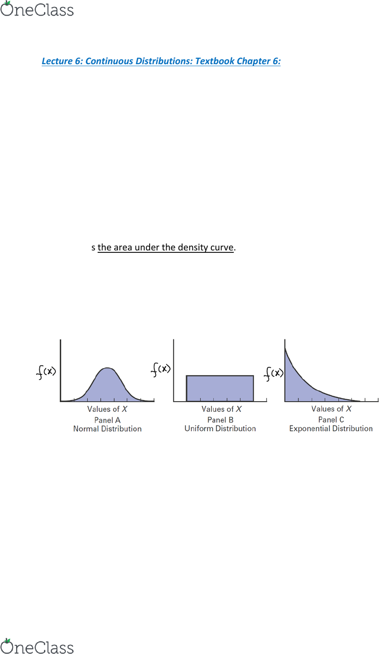
probability is the area under the density curve. The probability of the mean
occurring is also 0.
N.B. The probability of a specific value is 0 because it has no area under density curve
A probability density function is a mathematical expression that defines the
distribution of the values for a continuous variable. Graphed below are three
continuous probability density functions:
Panel A depicts a normal distribution. The normal distribution is symmetrical and
bell-shaped, implying that most observed values tend to cluster around the mean,
which, due to the distribution’s symmetrical shape, is equal to the median. Although
the values in a normal distribution can range from negative infinity to positive infinity
( + ), the shape of the distribution makes it very unlikely that extremely
large or extremely small values will occur.
Panel B shows a uniform distribution where the values are equally distributed in the
range between the smallest value and the largest value. Sometimes referred to as
the rectangular distribution, the uniform distribution is symmetrical, and therefore
the mean equals the median.
find more resources at oneclass.com
find more resources at oneclass.com
Panel C illustrates an exponential distribution. This distribution is skewed to the
right, making the mean larger than the median. The range for an exponential
distribution is zero to positive infinity, but the distribution’s shape makes it unlikely
that extremely large values will occur.
The Normal Distribution:
Panel A depicts a normal distribution. The normal distribution (also known as the
Gaussian distribution) is symmetrical and bell-shaped, implying that most observed
values tend to cluster around the mean, which, due to the distribution’s symmetrical
shape, is equal to the median. Although the values in a normal distribution can range
from negative infinity to positive infinity (-∞ to +∞), the shape of the distribution
makes it very unlikely that extremely large or extremely small values will occur.
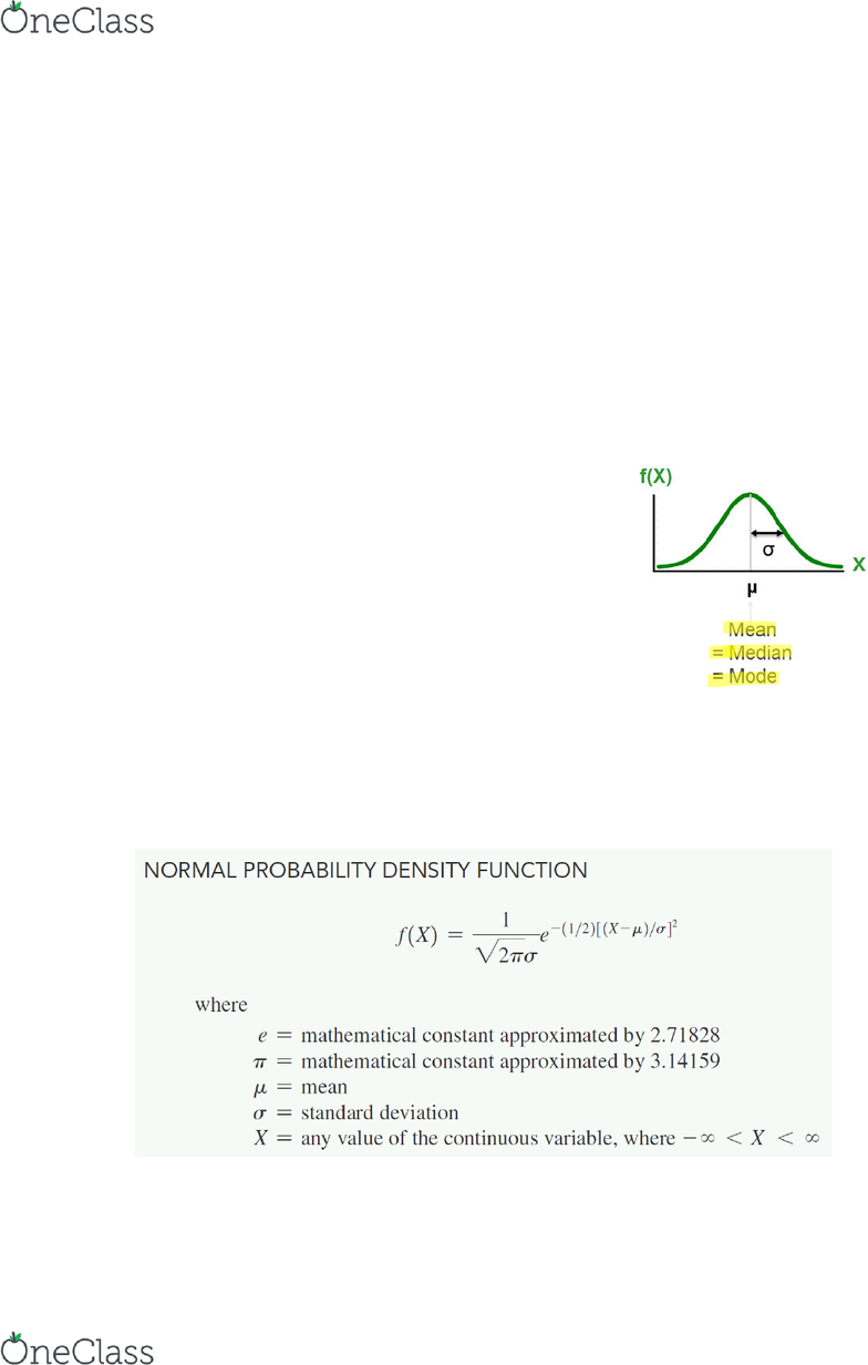
• Bell Shaped (skewness = 0, mean=mode=median)
• Symmetric
• Mean, Median and Mode are equal (or roughly equal)
• Location given by the mean parameter, μ.
• Spread given by the standard deviation parameter, σ.
• The random variable (rv) has an infinite theoretical
range: +∞ to – ∞ (Range ≅ 6σ)
• Its interquartile range is equal to 1.33 standard
deviations (≅ 1.33σ). Thus, the middle 50% of the values are contained within
an interval of two-thirds of a standard deviation below the mean and two-
thirds of a standard deviation above the mean.
The symbol f(X) is used to represent a probability density function:
By varying the parameters μ and σ, we can obtain different normal distributions:
find more resources at oneclass.com
find more resources at oneclass.com
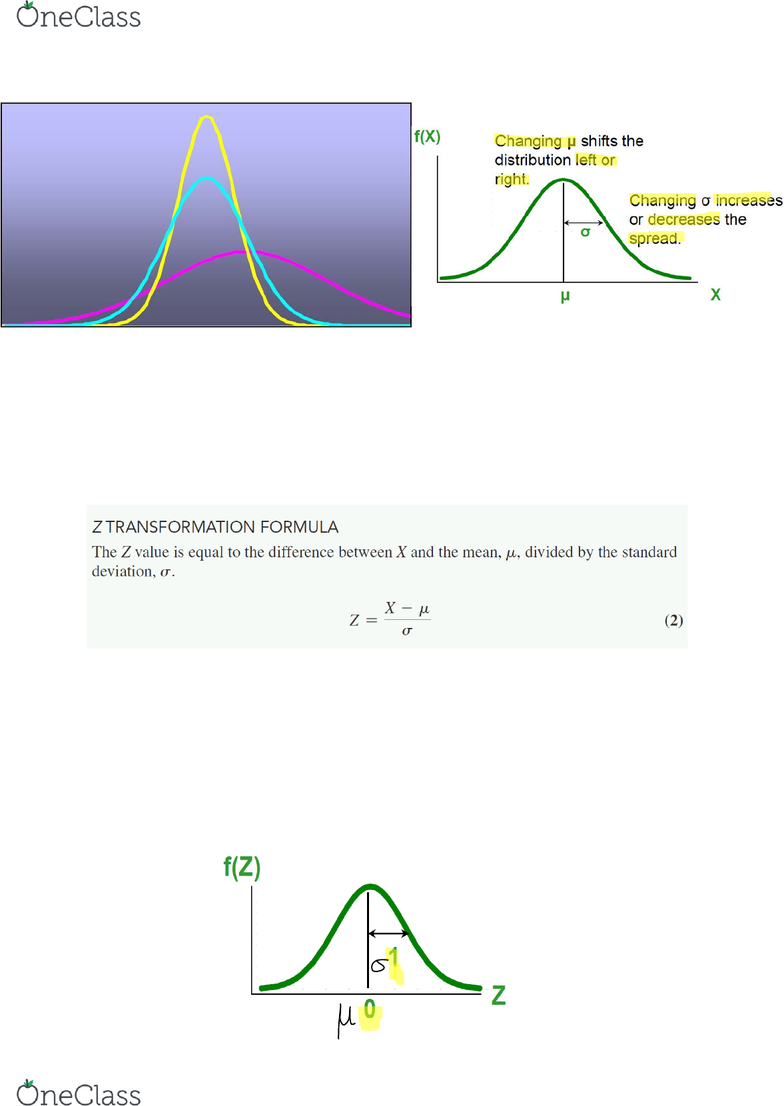
Computing Normal Probabilities:
To compute normal probabilities, you first convert a normally distributed variable, X,
to a standardised normal variable, Z, using the transformation formula. Applying this
formula allows you to look up values in a normal probability table and avoid the
tedious and complex computations that Equation (1) would otherwise require.
This is also known as the standardised normal distribution:
• Any normal distribution (with any mean and standard deviation combination)
can be transformed into the standardized normal distribution (Z).
• Needed to transform X units into Z units.
• The standardized normal distribution (Z) has a mean of 0 and a standard
deviation of 1.
• X values above the mean have positive Z-values, X values below the mean
have negative Z-values.
find more resources at oneclass.com
find more resources at oneclass.com

