MATH1005 Lecture Notes - Lecture 8: Central Limit Theorem, Probability Distribution, Normal Distribution

25 Oct 2018
School
Department
Course
Professor
Document Summary
This is one of the three histogram categories, with data and simulation. A data histogram is written with hist(); while the probability histogram is representative of chance, defined by area. Code: sum = c( 2 : 12 ) chance = c( 1 , 2 , 3 , 4 , 5 , 6 , 5 , 4 , 3 , 2 , 1 )/ 36 t = data. frame(sum, chance) barplot(t, names. arg = t, main = "probability histogram of sums" ) A simulation histogram would represent the same as the probability histogram, except, representing simulation of that change. The convergence of simulation histogram is actually related to the probability histogram. Take note: ev (expected value) = centre, se (standard error) = spread. This is where the probability histogram for the sum will closely follow the normal curve. It must meet certain conditions to be true.