ECON1203 Lecture Notes - Lecture 10: Null Hypothesis, Contingency Table, Test Statistic


9 – Chi-squared tests
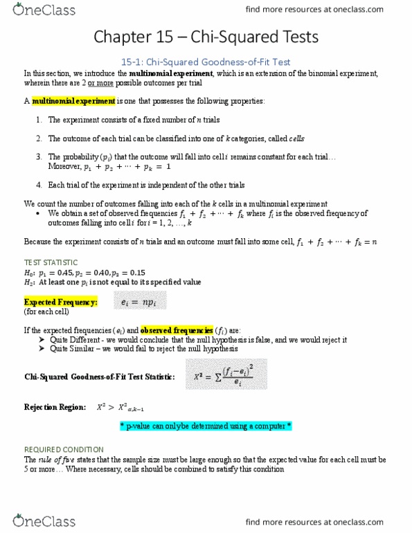
Chi-squared goodness-of-fit test – used to test the null hypothesis that the observed and
expected distributions are the same
• H0 specifies probability pi that an observation falls into i = , …, c categories or cells
H0 implies expected frequencies for a sample of size n (ei = pi n), assuming:
(a) Random sampling (independent trials)
(b) Probabilities pi are constant over trials
• The test can be unreliable if any ei = pi n is too small (e.g. 3 or 4)
Solution: merge categories together, where sensible
• The distribution theory underlying this test is not exact
It is large sample theory (a reason for the limitation about small expected cell
frequencies)
• The test statistic is given by:
• In other words, the statistic will be drawn from a Chi-squared distribution with c – 1
degrees of freedom, if the null hypothesis is correct
oi = observed frequency in cell i
ei = expected frequency in cell i
The 2 distribution
• An asymmetric distribution characterised by degrees of freedom, v
• Its support lies on the interval , ∞; it is exclusively non-negative
• It is the sum of the squares of v independent standard normal tables
• Gives the right-tail probability
• Because the support is non-negative and the curve is asymmetric, the tables for the
distribution must be used with care
Contingency tables
• Set up imaginary contingency table which assumes independence between the two
aspects under analysis
Use marginal (row and column) totals from the data to generate expected
frequencies for each cell
The expected frequency of observations in the cell in row i and column j under
independence is:
(a) where ni. = total observations in row i = , …, r
find more resources at oneclass.com
find more resources at oneclass.com