CAS EC 203 Lecture Notes - Lecture 12: Normal Distribution, Probability Distribution, Random Variable

Get access


Related Documents
Related Questions
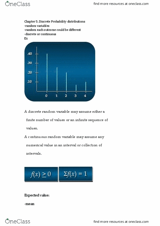
Consider a car owner who has an 80% chance of no accidents in a year. For simplicity, assume that there is a 10% probability that after the accident the car will need repairs costing $500, an 8% probability that the repairs will cost $5,000, and a 2% probability that the car will need to be replaced, which will cost
$15,000. Based on this information, the probability distribution, f(x), of the random variable, X, loss due to accident, is:
|
f(x) = |
|
0.8 x = $0 |
|
0.10 x = $500 |
|
0.08 x = $5,000 |
|
0.02 x = $15,000 |
where the first column is the probability of the event (i.e. P(x=0) =0.8) and the second is the severity.
Assuming risk retention, calculate the object risk to the car owner. Show ALL your work.
Now consider an insurance company that will reimburse repair costs resulting from accidents for 100 car owners, each with the same probabilities and losses as in part a). Calculate the objective risk for the insurance company. How is this number compared to that of part a)? Explain. Show ALL your work.
Suppose that the insurance company provides insurance to the same 100 car owners but now it introduces a deductible of $500. The claim payment distribution for EACH policy would now be:
|
f(y)= |
|
0.90 x = $0 or $500 y = $0 |
|
0.08 x = $5,000 y = $4,500 |
|
0.02 x = $15,000 y = $14,500 |
where


Problem 1
In each of the three games shown below, let p be the probability that player 1 plays cooperates (and 1- p the probability that player 1 defects), and let q be the probability that Player 2 plays cooperates (and 1- q the probability that player 2 defects).
Prisonerââ¬â¢s Dilemma
| Player 2 | |||
| Player 1 | cooperate | defect | |
| cooperate | 70,70 | 10,80 | |
| defect | 80,10 | 40,40 | |
Stag Hunt
| Player 2 | |||
| Player 1 | cooperate | defect | |
| cooperate | 70,70 | 5,40 | |
| defect | 40,5 | 40,40 | |
Chicken
| Player 2 | |||
| Player 1 | cooperate | defect | |
| cooperate | 70,70 | 50,80 | |
| defect | 80,50 | 40,40 | |
1. For each game, draw a graph with player 1ââ¬â¢s best response function (choice of p as a function of q), and player 2ââ¬â¢s best response function (choice of q as a function of p), with p on the horizontal axis and q on the vertical axis.
2. Using this graphs, find all the Nash equilibriums for the game, both pure and mixed strategy Nash equilibriums (if any). Label these equilibriums on the corresponding graph.
3. In those games that have multiple pure strategy Nash equilibriums, how do the expected payoffs from playing the mixed strategy Nash equilibrium compare with the payoffs from playing the pure strategy Nash equilibriums? Which type of strategy (mixed or pure) would players prefer to play in these games?
Problem 2
Two people are involved in a dispute. Player 1 does not know whether player 2 is strong or weak; she assigns probability ñ to player 2 being strong. Player 2 is fully informed. Each player can either fight or yield. Each player obtains a payoff of 0 is she yields (regardless of the other personââ¬â¢s action) and a payoff of 1 if she fights and her opponent yields. If both players fight, then their payoffs are (-1; 1) if player 2 is strong and (1;-1) if player 2 is weak. The Bayesian game is the following, depending on the type of player 2:
| Y | F | Y | F | ||||||
| Y | 0, 0 | 0, 1 | Y | 0, 0 | 0, 1 | ||||
| F | 1, 0 | -1, 1 | F | 1, 0 | 1, -1 | ||||
| Player 2 is strong (ñ) | Player 2 is weak (1-ñ) | Player 2 is strong (ñ) | |||||||
After writing all the strategies and payoffs in the same matrix, find the Bayesian Nash equilibriums, depending on the value of ñ (ñ ââ°Â¤ 1/2 or ñ ââ°Â¥1/2).
