ECON 6306 Lecture Notes - Lecture 11: Stochastic Process, Time Series, Stationary Process

12 May 2018
School
Department
Course
Professor

Generalized least squares
Till now we were talking about OLS ie ordinary least squares. But when we talked about the violations of
regression assumptions, OLS cannot be used directly to estimate the models. We need to make certain
adjustments. This method is called generalized least squares. The violations usually result in the
residuals not being identical and independent.
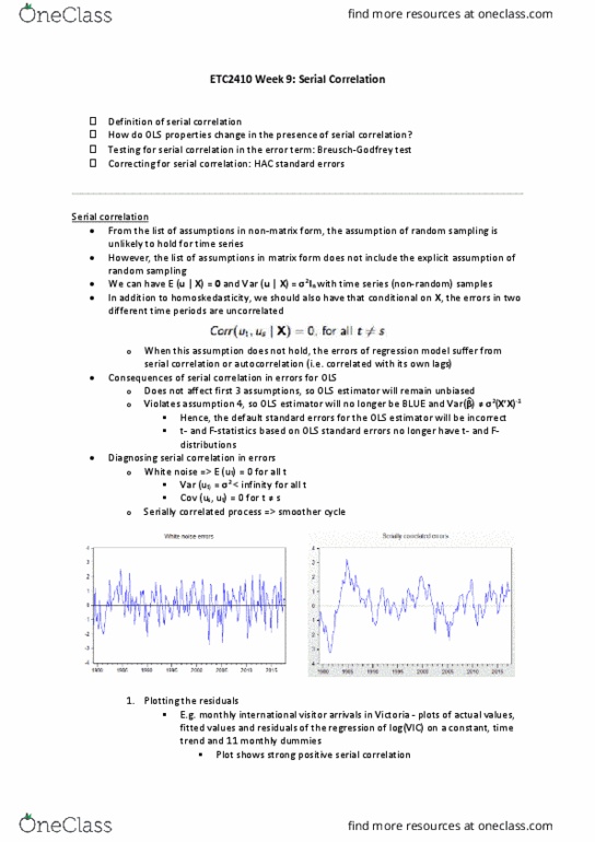
Serial Autocorrelation
Autocorrelation is found in time series data where residuals of one time period is correlated with
residuals from the time periods immediately preceding it.
A time series can be decomposed into two parts:
• The trend, seasonality or cyclic behavior. This is called the first order component and can be
modeled through our x variables.
• The remaining residuals have are a stochastic random process. Once we have tried to control for
the first order component, we try to model this second order component.
How to identify?
The statistic used to identify autocorrelation is called the Durbin Watson test. The code to run it is given
below:
library(lmtest)
dwtest(model1)
dwtest returns the D statistic. If D=2, then there is no autocorrelation. If D<2, then there is positive
autocorrelation, and if D>2, then there is negative autocorrelation.
Modeling autocorrelation
To model the stochastic process behind a time series, we divide it into two parts: moving average and
autoregressive parts. A model can have either of them or none or both.
Before starting the actual modeling process, we have to make our time series stationary with respect to
time.
In a stationary process the mean, variance and covariance are all stationary. If a series is non-stationary,
it can be made stationary by first differencing i.e. compute yt – yt-1 . See if this variable is stationary.
find more resources at oneclass.com
find more resources at oneclass.com
Document Summary
Till now we were talking about ols ie ordinary least squares. But when we talked about the violations of regression assumptions, ols cannot be used directly to estimate the models. The violations usually result in the residuals not being identical and independent. Autocorrelation is found in time series data where residuals of one time period is correlated with residuals from the time periods immediately preceding it. A time series can be decomposed into two parts: the trend, seasonality or cyclic behavior. This is called the first order component and can be modeled through our x variables: the remaining residuals have are a stochastic random process. Once we have tried to control for the first order component, we try to model this second order component. The statistic used to identify autocorrelation is called the durbin watson test. The code to run it is given below: library(lmtest) dwtest(model1) dwtest returns the d statistic.