STAT 3006 Lecture Notes - Fall 2018 Lecture 2 - Null hypothesis, Dependent and independent variables, Descriptive statistics

21 Sep 2018
School
Department
Course
Professor

Daniel T. Eisert STAT-3006
1
9.1 Inference for Two-Way Tables
Chapter IX: Analysis of Two-Way Tables
Inference for
Two-Way Tables
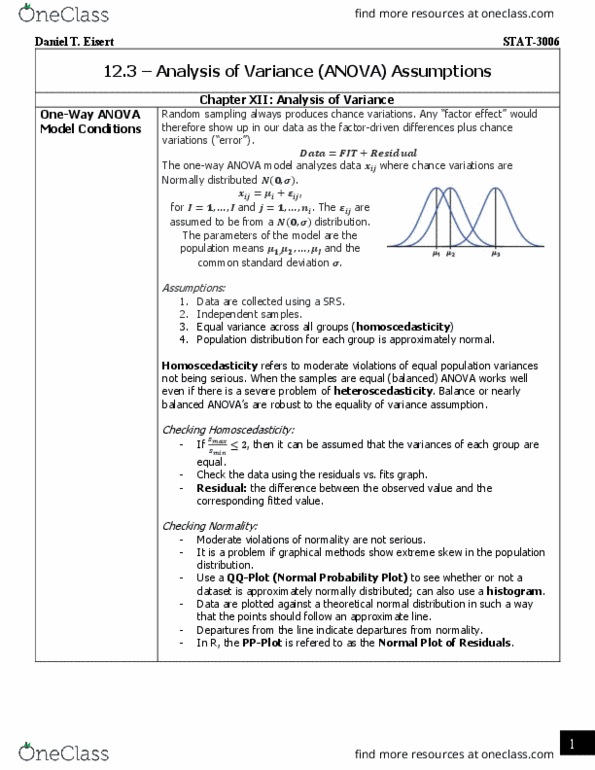
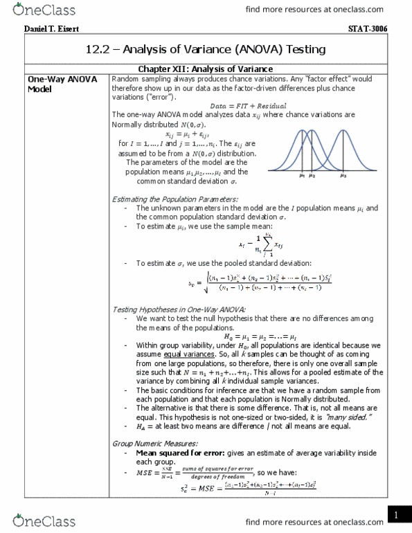
Recall ~ when the data are obtained from random sampling, two-way tables of
counts can be used to formally test the hypothesis that the two categorical
variables are independent in the population from which the data were
obtained.
- Joint Probability refers to dividing each cell entry by the total sample
size.
- Marginal probability is the probability distribution based on each
categorical variable.
- Conditional probability is the distribution of one variable when
conditioning on the value of the other variable.
Joint Probability Distribution
- Let X and Y be two discrete
random variables. The joint
probability function f(x, y) and X
and Y is defined by:
1. for all x og y
2. The sum of all x and y probabilities equals 1
3. The probability that both X = x and Y = x
x = 2
x = 4
TOTALS
Margins of Y
y = 1
0.1
0.15
0.25
y = 3
0.2
0.3
0.5
y = 5
0.1
0.15
0.25
TOTALS
Margins of X
0.4
0.6
1.0
Marginal Probability Function
X = S1, Y = S2
• Example: Based on the chart above, what is the marginal distribution of
x? →
Joint Distribution refers to two random variables X and Y with joint
density/probability functions f(x, y) and marginal density/probability
functions g(x) and h(y), respectively, are said to be independent if and only if
for all x, y.
Conditional Probability
- Let X and Y two random variables with join probability density
functions and marginal densities, then the conditional density of Y
given X = x is the following formula.

Daniel T. Eisert STAT-3006
2
Inference for
Two-Way Tables
Conditional Probability Formula
• EXAMPLE: Use the above. Notice there are two options for x, so we
need two cases.
Two cases:
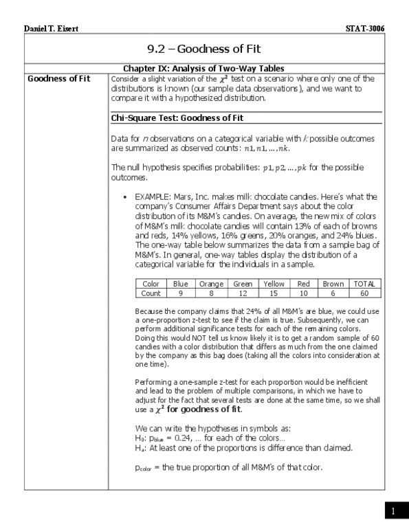
• EXAMPLE: Suppose you asked 20 children and adults whether they
liked broccoli. The joint relative frequencies are the value in each
category divided by the total number of values. The joint relative
probability would be each box divided by n or 20.
Yes
No
TOTALS
Children
3
8
11
Adults
7
2
9
TOTALS
10
10
20
Joint Probability
Yes
No
Children
0.15 (3/20)
0.40 (8/20)
Adults
0.35 (7/20)
0.10 (2/20)
Marginal Probability of Liking Broccoli
Yes
No
Proportion
0.50 (10/20)
0.50 (10/20)
Marginal Probability of Age (children or adults)
Children
Adults
Proportion
11/20
9/20
Conditional Probability of Liking Broccoli Given Being a Child
Yes
No
Proportion
3/11
8/11
Conditional Probability of Liking Broccoli Given Being an Adult
Yes
No
Proportion
7/9
2/9
Conditional Probability of Age Given Liking Broccoli
Yes
No
Proportion
3/10
7/10
Conditional Probability of Age Given Not Liking Broccoli
Yes
No
Proportion
8/10
2/10
Document Summary
Recall ~ when the data are obtained from random sampling, two-way tables of counts can be used to formally test the hypothesis that the two categorical variables are independent in the population from which the data were obtained. Joint probability refers to dividing each cell entry by the total sample size. Marginal probability is the probability distribution based on each categorical variable. Conditional probability is the distribution of one variable when conditioning on the value of the other variable. Let x and y be two discrete random variables. Joint distribution refers to two random variables x and y with joint density/probability functions f(x, y) and marginal density/probability functions g(x) and h(y), respectively, are said to be independent if and only if (cid:1858)(cid:4666)(cid:1876),(cid:1877)(cid:4667)=(cid:1859)(cid:4666)(cid:1876)(cid:4667) (cid:4666)(cid:1876)(cid:4667) for all x, y. Let x and y two random variables with join probability density functions and marginal densities, then the conditional density of y given x = x is the following formula.