STAT1008 Study Guide - Final Guide: Confidence Interval, Observational Error, Dependent And Independent Variables


Inference for Slope and Correlation
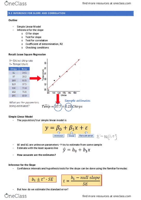
Simple Linear Model
• The population/true simple linear model is:
• 0 and 1 are unknown parameters.
• Estimate the least square line:
Inference for the Slope
• When the conditions for a simple linear model are reasonably met, we find:
Confidence Interval for Slope
• Confidence interval for the population slope =
• Where b1 is the slope for the least squares line for the sample and SE is the standard error of
the slope.
• t* uses n-2 degrees of freedom
T-Test For Correlation
• Test statistic:
• H0: 1 = 0 vs Ha: 1 0
• We are testing for the significance of the regression - "Is X an important predictor of Y".
• We estimate the SE with bootstrap/randomisation distributions.
• Bootstrap from the original data with replacement and fit the regression line to the new data.
Test for Slope
•
• Ho: 1=0 → no linear relationship
• Ha: 1 ≠0 (or 1-tail) → some relationship
•
• b1 and SE come from computer output.
• Find p-value using t-distribution with n-2 df.
Test for Correlation
• Ho: ρ=0
• Ha: ρ0 (or 1-tail)
•
• The t-test for slope and t-test for correlation are identical.
Coefficient of Determination, R2
• Recall that for correlation: -1 r 1.
• If we square the correlation, r2, we get a number between 0 and 1 that can be interpreted as a
percentage.
• R2 = proportion of variability in response variable Y that is "explained" by the model based on
the predictor X.
Checking Conditions for a Simple Linear Model
• For a simple linear model, we assume the errors (ε) are randomly distributed above and below
the line.
• Look at a scatterplot with regression line on it.
• Watch out for:
find more resources at oneclass.com
find more resources at oneclass.com
Document Summary
Confidence interval for slope the slope. t* uses n-2 degrees of freedom: the population/true simple linear model is, 0 and 1 are unknown parameters, estimate the least square line: (cid:1877) =(cid:2868)+(cid:2869)(cid:1876, confidence interval for the population slope = (cid:2869) . Test statistic: =(cid:3117) (cid:3041) (cid:3046)(cid:3042)(cid:3043: h0: 1 = 0 vs ha: 1 0, (cid:1877)=(cid:2868)+(cid:2869)(cid:1876)+ =(cid:3117: ho: =0, ha: 0 (or 1-tail) For a simple linear model, we assume the errors ( ) are randomly distributed above and below the line. 9. 2 anova for regression (analysis of variance: y=(cid:882)+(cid:883)+ data = model + error. 2 y (ssmodel) by the model: h0: (cid:2869)=(cid:882) (model is ineffective, hq: (cid:2869) (cid:882) (model is effective) F = msmodel/msw: to find a p-value for the anova f-statistic, create a randomisation distribution (keep one variable fixed and randomly reorder the other variable), or, use a theoretical distribution. F-distribution has degrees of freedom for both the numerator and the denominator.