ECON201 Study Guide - Midterm Guide: Diminishing Returns, Isoquant, Production Function
171 views4 pages

29 Apr 2013
School
Department
Course
Professor


15
ECON201 Full Course Notes
Verified Note
15 documents
Document Summary
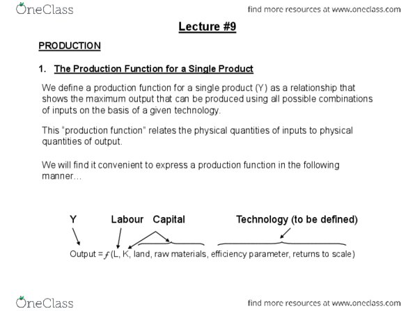
Production function: maximum output that can be produced using all possible combinations of inputs on the basis of a given technology. Output = f (l, k, land, raw materials, ef ciency parameter, returns to scale) Capital = k, land, raw materials; land and raw materials absorbed into k for analysis simplicity. Technology = ef ciency parameters, returns to scale; assume held constant. General form of production function: y = f (k, l) Short-run production function, marginal product, and average product. Short-run production function: labour variable, k and tech xed. Mp = slope of tpl (total product of labour), ap = y / l. As l (k constant) eventually mpl and apl . Realized when mpl and mpk are both positive. A process is technologically ef cient if it cannot be shown to be inef cient. Isoquant: locus of all technologically ef cient processes for producing a given quantity of output. Vertical and horizontal segments simply represent constant output.
Get access
Grade+20% off
$8 USD/m$10 USD/m
Billed $96 USD annually

Homework Help
Study Guides
Textbook Solutions
Class Notes
Textbook Notes
Booster Class
40 Verified Answers
Related Documents
Related Questions

The law of eventually diminishing marginal returns: (Points : 1)
a. states that each and every increase in the amount of the variable factor employed in the production process will yield diminishing marginal returns.
b. is a mathematical theorem that can be logically proved or disproved
c. is the rate at which one input may be substituted for another input in the production process
d. None of the above
b. the incremental change in total output that can be produced by the use of one more unit of the variable input in the production process c. the percentage change in output resulting from a given percentage change in the amount of the variable input X employed in the production process with Y d. None of the above |
b. the marginal rate of technical substitution c. equal to MPx/MPy d. all of the above e. none of the above |
b. equal to the marginal factor cost of the variable factor times the marginal revenue resulting from the increase in output obtained c. equal to the marginal product of the variable factor times the marginal product resulting from the increase in output obtained d. a and b e. a and c |
b. variable cost c. marginal rate of technical substitution d. total cost e. none of the above |
b. the average product of labor (L) is equal to ?2 c. if the amount of labor input (L) is increased by 1 percent, then output will increase by ?1 percent d. a and b e. a and c |
b. relevant to decisions in which one or more inputs to the production process are fixed c. not relevant to optimal pricing and production output decision facilities d. crucial in making optimal investment decisions in new production facilities e. none of the above |
b. all inputs are considered variable c. some inputs are always fixed d. capital and labor are always combined in fixed proportions |
| A linear total cost function implies that: (Points : 1) |
b. average total costs are continually decreasing as output increases
c. a and b
d. none of the above
