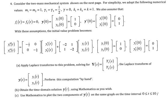
Consider the two-mass mechanical system shown on the next page. For simplicity, we adopt the following numerical values, m_1 = m_2 = 1, gamma_1 = gamma_2 = 1/2, y = 0, k_ 1 = k_2 = k =1. We also assume that: f_1(t) = f_2(t) = 0, y(0) = [y_1(0) y_2(0)] = [1 0], y'(0) = [y'_1(0) y'_2(0)]] [0 1]. With these assumptions, the initial value problem becomes: [y"_1(t) y"_2(t)] = [-1/2 0 0 -1/2] [y'_1(t) y'(2)] + [-2 1 1 -2] [y_1(t) y_2(t)], [y_1(0) y_2(0)] = [1 0], [y'_1(0) y'_2(0)] = [0 1] (a) Apply Laplace transforms to this problem, solving for Y(s) = [Y_1(s) Y_2(s)], the Laplace transform of y(t) = [y_1(t) y_2(t)]. Perform this computation "by hand". (b) Obtain the time-domain solution y (t), using Mathematica as you wish. (c) Use Mathematica to plot the two components of y(t) on the same graph on the time interval 0 lessthanorequalto t lessthanorequalto 10/
Show transcribed image text Consider the two-mass mechanical system shown on the next page. For simplicity, we adopt the following numerical values, m_1 = m_2 = 1, gamma_1 = gamma_2 = 1/2, y = 0, k_ 1 = k_2 = k =1. We also assume that: f_1(t) = f_2(t) = 0, y(0) = [y_1(0) y_2(0)] = [1 0], y'(0) = [y'_1(0) y'_2(0)]] [0 1]. With these assumptions, the initial value problem becomes: [y"_1(t) y"_2(t)] = [-1/2 0 0 -1/2] [y'_1(t) y'(2)] + [-2 1 1 -2] [y_1(t) y_2(t)], [y_1(0) y_2(0)] = [1 0], [y'_1(0) y'_2(0)] = [0 1] (a) Apply Laplace transforms to this problem, solving for Y(s) = [Y_1(s) Y_2(s)], the Laplace transform of y(t) = [y_1(t) y_2(t)]. Perform this computation "by hand". (b) Obtain the time-domain solution y (t), using Mathematica as you wish. (c) Use Mathematica to plot the two components of y(t) on the same graph on the time interval 0 lessthanorequalto t lessthanorequalto 10/