STA 101 Chapter Notes - Chapter Unit 7: Model Selection, F-Test, Multicollinearity

10 May 2018
School
Department
Course
Professor

Unit 7 Multiple Linear Regression
Part 1: (1) Multiple Predictors
Ex: weights of books, volumes (predictor), and type of cover (predictor)
Predicted weight = 197.96 + 0.72(volume) – 184.05(cover:pb)
For hardcover books: plug in 0 for cover
o Predicted weight = 197.96 + 0.72(volume)
o Started from a multiple regression model and simplified to a simple regression model
For paperback books, plug in 1 for cover
o Predicted weight = 13.91 + 0.72(volume)
Lines for paperback and hardcover books are parallel
Interpreting the regression parameters:
o Slope of volume: All else held constant, for each 1 cm3 increase in volume, the model
predicts the books to be heavier on average by 0.72 grams
o Slope of cover: All else held constant, the model predicts that paperback books weight
184.05 g lower than hardcover books, on average
o Intercept: Hardcover books with no volume are expected on average to weigh 198 grams
▪ Meaningless in context, serves to adjust the height of the line
Interaction variables
o Model assumes hardcover and paperback books have the same slope for the relationship
between their volume and weight
o If this isn’t reasonable, then we include an interaction variable in the model (beyond the
scope of this course) – just know that this simplying assumption doesn’t always make sense
Part 1: (2) Adjusted R2
Ex: Predicting % living in poverty from % of female householder
o R2 = 0.28
Ex: Predicting % living in poverty from % of female householder and % white
o Adding another explanatory variable doesn’t change SSTot since that is the inherent
variability in the response variable
o R2 = (SSfemale_house + SSwhite)/SSTot = 0.29
R2 value will go each time you add a predictor to your model
Adjusted R2: R2ADJ = 1 – ((SSE/SST)(n – 1/n – k – 1)); k = # of predictors; n = sample size
o Penalty for additional predictor included in the calculation, so instead of 0.29, we get 0.26
o When any variable is added to the model, R2 increases
o But if the added variable doesn’t really provide any new information, or is completely
unrelated, the adjusted R2 does not increase
Properties of Adjusted R2
o K is never negative adjusted R2 < R2
o Adjusted R2 applies a penalty for the number of predictors included in the model
o We choose models with higher adjusted R2 over others
Part 1: (3) Collinearity and Parsimony
Two predictor variables are said to be collinear when they are correlated with each other
o Remember: Predictors are also called independent variables, so they should be
independent of each other – so they shouldn’t be collinear
find more resources at oneclass.com
find more resources at oneclass.com

o Inclusion of collinear predictors (also called multicollinearity) complicates model
estimation – results from model may no longer be reliable
Parsimony: Avoid adding predictors associated with each other because the addition of such
variables brings nothing new to the table
o Prefer the simplest best model, i.e. the parsimonious model
▪ Occam’s razor: Among competing hypotheses, the one with the fewest assumptions
(or predictors in this case) should be selected
o Addition of collinear variables can result in biased estimates in the regression parameters
Part 2: (1) Inference for MLR
Determining which predictors are the significant predictors
Inference for the model as a whole
o Null: β1 = β2 = … = βk = 0
o Alt: At least one βi is different than 0
Since p-value < 0.05, the model as a whole is significant
o The F test yielding a significant result doesn’t mean the model fits the data well, it just
means at least one of the βs is non-zero
o The F test not yielding a significant result doesn’t mean individual variables included in the
model are not good predictors of y, it just means that the combination of these variables
doesn’t yield a good model
Afterwards, we can do individual hypothesis testing for slopes
o Is whether or not the mother went to high school a significant predictor of the cognitive
test scores of children, given all other variables in the model?
o Null: β1 = 0, when all other variables are included in the model
o Alt: β1 is not 0, when all other variables are included in the model
o We look at the p-value for that specific variable in the regression output
Testing for the slope – mechanics (understanding what the software is doing)
o T-statistic in inference for regression – T = (b1 – 0)/SEb1
o Df = n – k – 1; k = # of predictors
Confidence intervals for slopes
o b1 plus or minus (t*)(SEb1)
Interpretation of confident interval:
o CI: (-2.09, 7.17)
o We are 95% confident that, all else being equal, the model predicts that children whose
moms work during the first 3 years of their lives score 2.09 points lower to 7.17 points
higher than those whose moms did not work.
Part 3: (1) Model Selection
Stepwise model selection
o Backwards elimination: start with a full model (containing all predictors), drop on
predictor at a time until the parsimonious model is reached
o Forward selection: start with an empty model and add one predictor at a time until the
parsimonious model is reached
o Criteria:
▪ P-value, adjusted R2
▪ AIC, BIC, DIC, Bayes factor, Mallow’s Cp (beyond the scope of this course)
Backwards elimination – adjusted R2
o Start with the full model
o Drop one variable at a time and record the adjusted R2 of each smaller model
o Pick the model with the highest increase in adjusted R2
find more resources at oneclass.com
find more resources at oneclass.com
Document Summary
Ex: weights of books, volumes (predictor), and type of cover (predictor) Predicted weight = 197. 96 + 0. 72(volume) 184. 05(cover:pb) For hardcover books: plug in 0 for cover: predicted weight = 197. 96 + 0. 72(volume, started from a multiple regression model and simplified to a simple regression model. For paperback books, plug in 1 for cover: predicted weight = 13. 91 + 0. 72(volume) Lines for paperback and hardcover books are parallel. 184. 05 g lower than hardcover books, on average: intercept: hardcover books with no volume are expected on average to weigh 198 grams, meaningless in context, serves to adjust the height of the line. Part 1: (2) adjusted r2: r2 = 0. 28 between their volume and weight. Ex: predicting % living in poverty from % of female householder: model assumes hardcover and paperback books have the same slope for the relationship. R2 value will go each time you add a predictor to your model unrelated, the adjusted r2 does not increase.