ECO102H1 Lecture 33: Lecture 33-Shifts in Aggregate Supply Curve


=/='=y[- M
Y0[
Desired
Spending
45°
Real income (Y)
Y0
C + I + G + X - M
10
Tuesday, February 23rd, 2010.
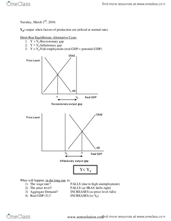
Shifts in Aggregate Supply
Remember
1. 65$6UHODWLRQEHWZHHQUHDO*'3ILUP¶VGHVLUHGSURGXFWLRQ´DQGSULFHOHYHOwhen
prices of factors of production (including wages) are constant
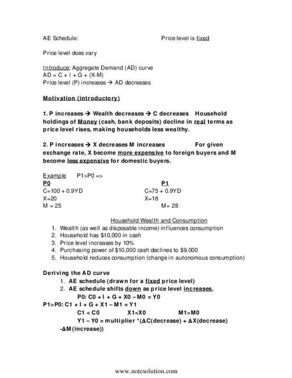
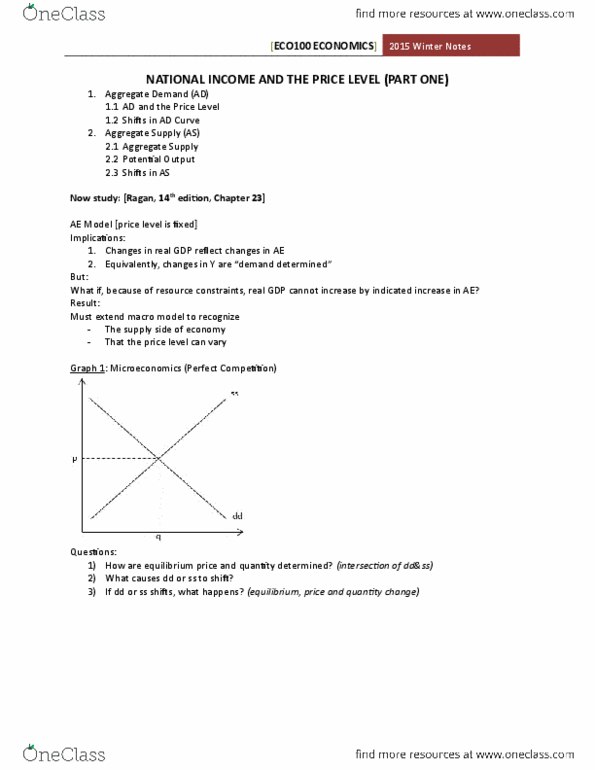
2. AD: relation between desired spending and price level
Change in Macroeconomic Equilibrium
1. 6KLIWLQ$'³GHPDQGVKRFN´
Increase in autonomous expenditure shifts AD to right.
Price level 9UHDO*'39
Example: Exports (X) increase by $10 billion
Step One: Price Level is Fixed
Y0¶± Y0 = multiplier * change in autonomous expenditure
= 2 * 10 = 20 (if multiplier = 2)
Step Two: Price Level can Vary
=/='=y[- M
Y0[
Desired
Spending
45°
Real income (Y)
Y0
C + I + G + X - M
10
www.notesolution.com


45
ECO102H1 Full Course Notes
Verified Note
45 documents