Statistical Sciences 2244A/B Lecture Notes - Lecture 11: Binomial Distribution, Color Blindness, Random Variable

17 views4 pages

tealminnow441

22 May 2018

School

Western University

Department

Statistical Sciences

Course

Statistical Sciences 2244A/B

Professor

Jennifer Waugh

For unlimited access to Class Notes, a Class+ subscription is required.

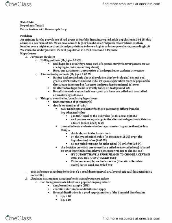
Stats 2244

Hypothesis Tests I

Introduction to P values

The Problem

- If we had a sex biased population (more of one sex), you might expect a higher proportion of

red/green blindness depending on the sex ratio

- ANSWER: B

o Reasonable to predict a lower proportion bc we have a previous reason to expect it to be

less

o males are more likely to have red green color blindness than females – so if we have

fewer males than what is expected, then it can be reasonable to assume P<0.0425

- ANSWER:

o The sample size should make our estimate a better approximation of the parameter

o Larger samples result in sample means that are closer to the population mean (same

thing is true about proportions)

o The key thing about the p hat value is that its a statistic

▪ A statistic is never a definitve value – they just describe samples

▪ The value you get for your statistic depends on the sample you take!!

▪ This makes us say that we dont have enough yet

o Remember that this is one sample from the population and its one statistic in a whole

possibility of statistics

o We could have just as easily got a sample with 10 successes out of 200 →this would

have gave us a sample proportion (p hat) of 0.5

o We know that sample size influences the variation in the possible statistic (recall the

formula for the sigma of proportinos)

o When you take a single sample and get a single sample estimate – we have to think

about the sampling variability and how likely we are to get a value like that

find more resources at oneclass.com

Unlock document

This preview shows page 1 of the document.
Unlock all 4 pages and 3 million more documents.

Already have an account? Log in

Document Summary

If we had a sex biased population (more of one sex), you might expect a higher proportion of red/green blindness depending on the sex ratio. This is a binomial distribution with 200 trials and a probability of success of 0. 0425. Using r, we can calculate the probability that we get proportion of 0. 02, 4 times (we can also do this ourselves) The likelihood of going into this population and getting a sample where 4 of them are red green colour bind is 0. 02. You don(cid:495)t expect to get anything more than (cid:884)(cid:882) (cid:523)bc looking at the graph, the probability of. We have to have a way to juddge where the values that are likely are location getting those is small: we can use relative position (where you are relative to something else) Including 0, that makes 201: the discrete value that this variable could take on is (cid:882),(cid:883),(cid:884),(cid:885),(cid:886),(cid:887) (cid:884)(cid:882)(cid:882)

Related Questions

9. Write a method with the following header public static void replace (String oldFile, string newfile, char oldChar, char newChar) throws IOException This method opens the file whose name is given by the String parameter oldFile (the input file) for reading, and opens the file whose name is given by the string parameter newlile (the output file) for writing. It then reads every lime in the input file. For each line, it creates a new line identical to the original line, creept for the fact that all occurrences of char oldchar in the original String have been replaced by occurrences of char newchar in the new line. When the new line has been properly created, it write it to the output file. Once all the lines in the input file have been read and a corresponding line has been written to the output file, the method clases both files. Additional notes: • You MAY assume that none of the parameters this method accepts are null; in other words, your method does not have to handle the case where one or more of the parameters are null. You MAY assume that all the 10-related classes have already heen imported properly . Finally, because the replace() method is specified to throw an exception object of type TORxception, you MAY assume that I/O related problems will occur while reading from the input file or writing to the output file. In other words, your method DOES NOT have to check that no such problems occur, and DOES NOT have to manage Texceptions using try-catch blocks. WRITE YOUR replace() METHOD IN THE SPACE BELOW: YOUR replace() METHOD CONTINUED: USE THIS PAGE IF YOU NEED ADDITIONAL SPACE. CLEARLY INDICATE WHICH QUESTION(S) YOU ARE ANSWERING HERE. USE THIS PAGE IF YOU NEED MORE ADDITIONAL SPACE. CLEARLY INDICATE WHICH QUES- TION(S) YOU ARE ANSWERING HERE. • String (package java.lang) Methods: - public String chal wale Al t ri g od med in the chance au - public int length(): R e ach of the string - public char chattin R echar w heefd index public chart to Chachay: Consthis String to a new c r y - public boolean equals Object anbject): Ce this string to and yect - public boolean equalsigmoce Case String anotherstring]: Cam p ing sider this String to anotherString - public int compareToString anotherString: Compare this String to anotherstring graphically returns a negative ef this string before anotherstring, apithe value of this Stringatering distries publie iw paneelgoro (String another Camp i ng Garden ces, string to anoth i ng li hically returns te value of this thing care anotherstring, apie as if this string e r anotherstring, Strings - public int indexin ch Rather within this string of the och ch-lil does not - public int index fint.ch, int from index): Returns the index within this string of the first Roe of character ch, starting the search at position from Index retums - 1 il ch does not in this String - public int indexor (String ste): Returns the index within this string of the first currence of ringt-d eur - public int indexOf(stringate, int from index): Resures the index within the string of the fare currence of shariaparting police froiden liste des not count i ng - public String subat ring it begintndax) Rema new string which is a webstring of this string compend of the chesting at position begintndex (inclusive) - puble string subat ring intaginindex intendindex: Returns a new sering that waring of this string, composed of the characters starting at position beginIndex (inclusive, and ending at - public String replace(char oldChar, char newchar): Returns a new string resulting from replacing a Tences of olchar in this string with new Char. puble string tolon Case(): Returns a new string consisting of all the characters in this sting - publle ting toppe : Roum ingiting of all the c on in this thing uverted to perce - publie ting tet): Returns a copy of this line with leading and wailing whitespace • Scanner (package java.util) Methods: - publie danner File source) thrown jatorio Foundation sa Scanner the fun the specified file - public scanner InputStream source): Cits Scanner that process and from the input stream - puble Scannerstag source): Corsa ww Scanner that produces wales w ed from the specified String -puble vold close(): Cwes this Scanner -puble boolean asext(): Return this can het in its input puble boolean asext.Double(): Return to the taken in this season al ante pasadala w ith Doble() ed publie boolean hat Into: Reutte le inse gule ed wat w eet Int() had - public boolean hati : Return true if this w ee - puble boolean has longt) Return true if the r in this cannerm ane das along the next long) with puble ting at the t e rm from the canner puble double Smerthea ter puble intention there the l ot. puble w ith the need them - puble Intolog m u long • Printstream ( kape Java.io) Methods: a - Pri le rlle) throw alo.Pilo t Pelat ihan the p rile - Printing the throw r alo. Pet Stichw e d the wind - le void lose them - le void phone boolean ve - void prichar public void print chart 6): the way of char public void print double d o uble bed, public void print (int ) Fins int value - public void printet a n net public void printing : Strings - public void printin (1 Tm the line by writing the line para ring - public void printinhoolna ) Prints hoolean when thinorminates the public void printin (cthar c h ar wheelthening the line public void print in char i ta way of cars and then the line public void print in double d in double valued and the terminates the line public void printin(int 1) Pints int value and then into the line public void printin ( jat ova t terminates the line pulle void print intring): Tits Strings then to the line Note that the printwriter class defines the same methods and constructors (except for the fact that the structors are called Print.writer instead of PrintStream) • Math (package java.lang) Methods: - please le podle double bear the value of a t the of - puble balle blanche a Returns they u se of dele with pe r than realto - pietate double random Ruma doble 0.0 wi th .. puble stat la doble sin double a: Rethe puble statie doble con double a Return ther l e, where a ininin we angle, wherea in in e -puble statie doble tan double a) R he i ngold , whereas o m public statie double toeges double agrad): C a ngrad v ideo puble salle de anable and we a r e - - estatie delle au t olewa idle de ahholooble • Character (packape java.lang) Methods: - public static boolean ibigit charch: D i chtechisadil public static int digit(charch, int radix: Return the meal of cho ch in the di radix-lich des representa digit - public statie char forbigit chat digit, ut radix) Rems the character of digit in the disa - public statie boolean isletter charch): Demines if character chalet publle statie boolean islowerCase(char ch): Determines if character ch is a character - public static boolean ipparate(char eh): Determines ir ductes chinuppercase cura nd - publicatie boliwhip (arch Termine if character his white a intola - public static char tolowrane(char chevert hech to low - public static char tolpperCase(char ch): Covers Chococh topp • Array list (package java.util) Methods: - public ArrayList(): Create a new em ArrayList which contains clements of type - public int (1 : R m the number of clans in this list - public boolean isimpty(): Rens true if this in contains no elements - public boolean contains (object o): Return true if this lintutins el compr a re performed using the equals() method on - public int IndexOf(obj ): Returns the index of the first currence of elemento in this list, or lir this listes contain this element companies are performed wing the equals() method - publiek galimt in ): Returns the elementat position index in this list - publieket fint inde element): Replace the element at the position index in this list with the - puble honlanad a ): Appends the specifiedalent to the end of this list. - public void (int in aw e t the specified element the price index in this - publiek veint index): Remove the de s ition index in the list - publie hoolean remove(object a s the fir e of the president of this if it is p r epared wing the equals() methodno - public void clear(): Remes all of the elements from this • Vile (package java.io) Methods: - puble File(String pathname: Creates a File representing the file at the given pathane

Statistical Sciences 2244A/B Lecture Notes - Lecture 11: Binomial Distribution, Color Blindness, Random Variable

Document Summary

Get access

Related Documents

Statistical Sciences 2244A/B Lecture Notes - Lecture 12: Null Hypothesis, Simple Random Sample, Inference

Statistical Sciences 2244A/B Chapter Notes - Chapter 13: Estimation Theory, Central Limit Theorem, Bias Of An Estimator

Statistical Sciences 2244A/B Chapter Notes - Chapter 13,14: Statistical Inference, Sample Size Determination, Normal Distribution

Related Questions