STAT1008 Study Guide - Final Guide: Simple Random Sample, Dependent And Independent Variables, Bar Chart


1.Collecting data
Cases/units->row & variables->column
Categorical variable : divides cases into groups.
Quantitative variable : measures/records numerical quantity.
Explanatory var. helps understand/predict response var.
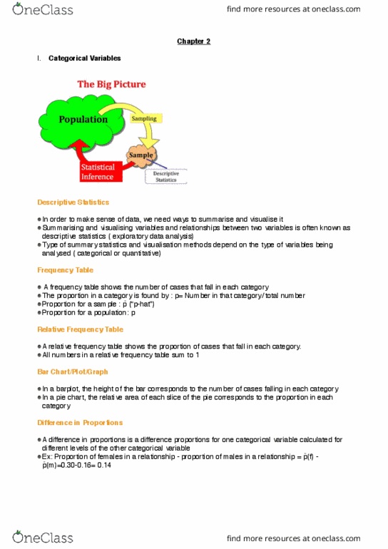
1.2 Sampling from a population
Pop = all individuals or objects of interest.
data collected from a sample = subset of pop. size of sample : n
Statistical inference = process of using data from a sample to gain
information about pop.
Bias exists when the method of collecting data causes the sample data to
inaccurately reflect the pop.
Sampling bias occurs when the method of selecting sample causes it to
differ from pop.
In a simple random sample of n units, all groups of size n in the pop have
the same chance of becoming the sample.-> avoids sampling bias
1.3 Experiments and observational studies
Two variables are associated if values of one variable tend to be related to
the values of the other variable.
Two variables are causally associated if changing the value of one variable
influences the value of the other variable.
Confounding variable/factor/lurking variable = third variable associated with
the explanatory and response variables.
If confounding vars are present a causal ass. can’t be determined
Experiment = study in which researcher controls one or more of the
explanatory variables
Observational study = researcher simply observes the values as they
naturally exist
-> they can almost never be used to establish causality.
In a randomised experiment the value of the explanatory variable for each
unit is determined randomly, before the response variable is measured.
Sample randomly selected ?
yes : possible to generalise to entire pop
no : cannot generalise
Explanatory variable randomly selected ?
yes : possible to make conclusions about causality
no : cannot make conclusions about causality
Types of randomised experiments :
1. randomised comparative experiment : randomly assign cases to
different treatment groups and then compare results on the
response variable(s)
2. matched paired experiment : each case gets both treatments in
random order and we examine individual differences in the response
variable between the two treatments
Control groups provide good comparison.
People who believe they are getting a treatment may experience desired
effects regardless of whether the treatment works -> placebo effect
2.1 Categorical variables
Proportion (=relative frequencies) in some category = Number in that category/Total
number
visualising proportions : bar chart, pie chart
Two way table used to show relationship between two categorical variables
visualising relationship between two categorical variables : segmented bar chart, side-
by-side bar chart
2.2 One quantitative variable : shape and center
Visualise distribution : dot plot, histogram
Shapes of distributions :
symmetric, skewed to the right, skewed to the left, bell shaped
Outlier : observed value that is notably distinct from the other values in a dataset.
Mean = Σx/n
Median m :
- middle entry if an ordered list of data values contains an odd number of entries
-average of the middle two values if even number
Resistance : a statistic is resistant if it is relatively unaffected by extreme
values
median, IQR = resistant / mean, s.d ≠ not resistant
skewed left : mean<median
skewed right : mean>median
symmetric : mean=median
2.3 One quantitative variable : measures of spread
Standard deviation measures the spread of the data in a sample. It gives a
rough estimate of the typical distance of a data value from the mean. The
larger the s.d the more variability there is in the data and the more spread
out the data are.
S.d and 95% rule
If distribution symmetric and bell-shaped, about 95% of the data should fall
within two s.d of the mean: x̅-2s and x̅+2s
Z-scores = (x- x̅)/s or (x-μ)/σ
z-score tells how many s.d the value is from the mean.
If data is symmetric and bell shaped about 95% of the data will fall within 2
s.d of the mean = only 5% of the data values will have z-scores beyond
+/-2
Percentiles
The Pth percentile is the value of a quantitative variable which is greater
than P percent of the data.
Five number summary = (min, Q1 (25th P), median, Q3 (75th P), max)
Range = max-min
IQR = Q3-Q1
2.4 Outliers, box plots, quantitative/categorical relationships
Outlier rule : < Q1-1.5(IQR) or > Q3+1.5(IQR)
Boxplots :
1)draw scale 2)draw box from Q1 to Q3 3)Draw line at the median 4)draw
line from quartile to last non outlier value 5)identify outlier with star
2.5 Two quantitative variables : scatterplot and correlation
Scatterplot : graph of the relationship between two quantitative variables.
Correlation : measure of the strength and direction of linear association
between two quantitative variables.
Properties :
-1 ⋜ r ⋜ 1, the sign indicates the direction of association, values close to
-1&1 have a strong linear relationship, r has no units, correlation is
symmetric between x&y.
3.1 Sampling distributions
Statistical inference : process of drawing conclusions about the entire population based on
the information in a sample.
Parameter : number that describes some aspect of a pop
Statistic : number that is computed from the data in a sample
We use the statistic from a sample as a point estimate for a pop parameter.
Sampling distribution : distribution of sample statistics computed for different samples of the
same size from the same population. Shows how the sample statistic varies from sample to
sample.
If samples are selected randomly and the sample size is big enough, the sampling
distribution will be symmetric and bell-shaped and centred at the value of the pop
parameter.
SE of a statistic is the SD of the sample statistic.
As sample size increase, the variability of sample statistics tend to decrease and sample
statistics tend to be closer to the true value of the pop parameter.
3.2 Confidence Intervals
An interval estimate gives a range of plausible values for a population parameter : Point
estimate +/- margin of error, where margin of error reflects the precision of the sample
statistic as a point estimate for this parameter.
Confidence interval for a parameter is an interval computed from sample data by a method
that will capture the parameter for a specified proportion of all samples.
The success rate = the confidence level
95% confidence interval can be estimated using :
Statistic +/- 2SE
3.3 Constructing bootstrap confidence intervals
-Generate bootstrap sample by sampling with replacement from the original sample
using the same sample size
-Compute statistic of interest called a bootstrap statistic for each of the bootstrap
samples
-Collect the statistics for many bootstrap samples to create a bootstrap distribution
SD of the bootstrap statistics in a bootstrap distribution gives a good approximation of the
SE of the statistic
If bootstrap distribution for a sample statistic is symmetric and bell-shaped, we estimate a
95% ci : statistic +/-2SE
3.4 Bootstrap CI using percentiles
If distribution approximately symmetric and bell shaped, we construct a ci by finding the
percentiles in the bootstrap distribution so that the proportion of bootstrap statistics
between the percentiles matches the desired confidence level
Larger sample sizes tend to increase the accuracy of the estimate, giving a smaller SE &
reducing the width of a confidence interval.
Document Summary
Pop = all individuals or objects of interest. data collected from a sample = subset of pop. size of sample : n. Statistical inference = process of using data from a sample to gain information about pop. Bias exists when the method of collecting data causes the sample data to inaccurately re ect the pop. Sampling bias occurs when the method of selecting sample causes it to differ from pop. In a simple random sample of n units, all groups of size n in the pop have the same chance of becoming the sample. -> avoids sampling bias. Two variables are associated if values of one variable tend to be related to the values of the other variable. Two variables are causally associated if changing the value of one variable in uences the value of the other variable. Confounding variable/factor/lurking variable = third variable associated with the explanatory and response variables.