ECO220Y1 Lecture Notes - Lecture 6: Sample Space, Empty Set


ECO220
Lecture 6
May 23, 2018
1
Ch. 7: Introduction to Simple Regression (Cont.)
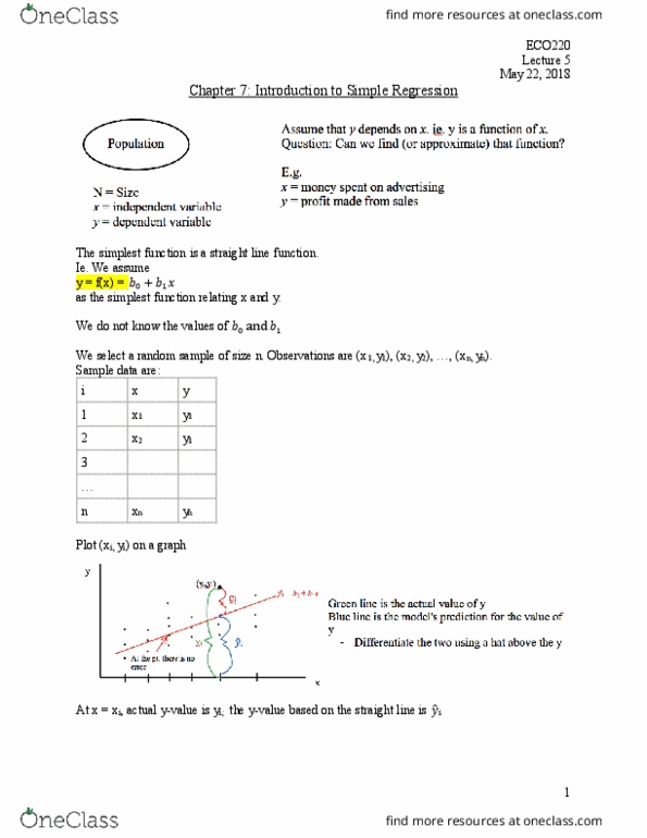
This model is a simple regression (straight line) model
and are unknown, but they have fixed values.
Select a sample of size n. Data are
x1, x2 … xn
y1, y2 … yn
Method of Ordinary Least Squares (OLS), we can calculate the estimates of and , called
and .
Note that and are sample statistics, their values will change from sample to sample.
The calculations of and are given in the Formula Sheet.
The regression equation is
ANOVA Table
From Lecture 5,
SST = SSR + SSE
• If =
, there is no error and SST = SSR
• However, this is often not the case in real life. There is usually an error (residual)
• If SSR is large, SSE will be small (and vice versa)
ANOVA Table
SS
df (degrees of
freedom)
MS (mean square)
F
Regression
SSR
1
MSR
MSR/MSE
Error
(Residual)
SSE
n-2
MSE
Total
SST
n-1
Where
,
Define R2 = Coefficient of determination
= % of variations in y that are explained by x.
Example 1: Let n=8 be a sample from a population. Sample observations are given in 2018-05-
23 Lecture 6 - Example. The estimated regression line is
= 15.7 - 0.126x

ECO220
Lecture 6
May 23, 2018
2
We can also calculate the correlation coefficient.
r = -0.94
(a) What is the coefficient of determination (R2)? Explain its meaning
R2 = (-0.94)2 = 0.89
89% of the variations in y can be explained by x.
The remaining 11% is the error --> Is not explained by the linear model
(b) Find SST
=(12.4 - 10.15)2 +… + (7.5 - 10.15)2
= 25.18
(c) Find the ANOVA Table
SS
df
MS
F
Regression
22.35
1
22.35
Error
2.83
6
0.47
Total
25.18
7
Since R2 =
, 0.89 =
, SSR = 22.35
Note: In our course, we use R2 and r2 interchangeably. i.e. we assume
R2 = r2
(d) You can calculate b1 from r
Test 1 Material Ends Here


27
ECO220Y1 Full Course Notes
Verified Note
27 documents
Document Summary
This model is a simple regression (straight line) model. Select a sample of size n. data are x1, x2 xn y1, y2 yn (cid:2868) and (cid:2869)are unknown, but they have fixed values. Method of ordinary least squares (ols), we can calculate the estimates of (cid:2868) and (cid:2869), called (cid:2868) and (cid:2869). Note that (cid:2868) and (cid:2869) are sample statistics, their values will change from sample to sample. The calculations of (cid:2868) and (cid:2869)are given in the formula sheet. If (cid:1877)= (cid:1877) , there is no error and sst = ssr: however, this is often not the case in real life. If ssr is large, sse will be small (and vice versa) Define r2 = coefficient of determination=(cid:3020)(cid:3020)(cid:3019)(cid:3020)(cid:3020)(cid:3021) = % of variations in y that are explained by x. (cid:1877) = 15. 7 - 0. 126x. Example 1: let n=8 be a sample from a population. 89% of the variations in y can be explained by x.